This tutorial is designed to walk users through the process of conducting a Power Analysis for the Classical Twin Design. To download the functions used on this website, you can right click on the icon![]() . To download the script to conduct the power analyses discussed on the website, you can right click on this icon
. To download the script to conduct the power analyses discussed on the website, you can right click on this icon ![]() . If you would like to follow the tutorials on your own computer, users should create a directory on their computer and save both files in that directory.
. If you would like to follow the tutorials on your own computer, users should create a directory on their computer and save both files in that directory.
The functions to conduct the power analysis are written in R, and use OpenMx to calculate the necessary statistics. The steps to obtain the required software are described in the next section.
R is a free, open source software program. R can be downloaded by clicking on the R icon. 

To calculate power in twin studies, we use OpenMx, an open-source software package that fits a variety of advanced multivariate statistical models. You can learn more about OpenMx by clicking on the OpenMx Guineapig. There are two ways to install OpenMx on your computer. First, open your R console. Then paste one of the following lines of code into the terminal window:
source('http://openmx.psyc.virginia.edu/getOpenMx.R')
While there are subtle differences between the versions of OpenMx, most users will not notice anything.
The figure presents a graphical depiction of primary components of statistical power. The standard power figure utilizing the normal distribution is presented in the left panel. This is the figure shown in most discussions of statistical power. The right panel is the analogous figure for the chi square distribution. While the figures appear to be starkly different, statistical power operates the same way for either distribution.
Because Likelihood Ratio Tests (LRTs) are the primary method of hypothesis testing for twin analyses, and the LRTs rely on the chi square distribution, it is necessary to discuss power from the perspective of the chi square distribution for the current purpose.
For both panels, the red distribution represents the distribution of test statistics assuming the null hypothesis is true while the blue distribution represents the distribution of test statistics assuming that the alternative hypothesis is true. The black line indicates the significance threshold (or α). The hatched red lines indicate the probably of rejecting the null hypothesis when the null hypothesis is true (a Type I Error). The hatched blue lines indicate the probably of failing to reject the null hypothesis, when the alternative hypothesis is true (a Type II Error). Power is the area under the alternative (blue) distribution that is not hatched. From this perspective the non-centrality parameter (ncp), is the parameter of interest.
There are two features of the ncp that are integral to the current discussion. First, as the effect size gets larger, the mean of the test statistic gets larger, and the ncp gets larger. Second, as sample size increases, the standard deviation of the sampling distribution of the test statistic gets smaller, and the ncp gets larger. Intuitively, it should make sense that power will increase (and the blue hatched area will decrease) with both larger effect sizes and larger sample sizes.
The current discussion uses 4 steps to calculate power:
- Simulate data for the MZ and DZ twins. The first step is to simulate twin data that corresponds with your expectations about the results. These expectations should be based, as far possible, on the literature. Of course, if you are doing something that has never been done before, these expectations can be less clear. It is also important to consider the ratio of MZ to DZ twins, as the power to detect significant genetic or environmental variance is influenced by this ratio. Specifically, you will need to provide the proportions of variance for the standardized A, C and E variance components. You will not have to simulate the data yourself (the functions will automatically take care of this step), but you will have to provide the values for the ACE parameters.
- Fit the model. The second step is simply to fit the model to the simulated data. Again, the function will do this automatically and return a set of fitted parameters. It is important to make sure that the fitted parameters correspond to the values that you specified in the previous stage. In some cases the simulated values may not correspond with the fitted parameters. In these cases, a warning message will appear. If this happens, it is possible to increase the sample size (keeping the ratio of the MZ to DZ twins constant). While fitting the full ACE model, it is trivial to also fit a reduced model where the parameter of interest is fixed to zero. Fitting both the full and the reduced model provides the difference between the -2 LogLikelihoods and the and obtain the χ2 value for the models, which is the primary purpose of this step.
- Obtain the weighted ncp (Wncp) Third, to obtain the Wncp, we divide the χ2 value by the total sample size (NMZ + NDZ). By dividing the χ2 value by the sample size, we are calculating the average contribution of each family to χ2 value. Therefore, this value is dubbed the weighted ncp (Wncp).
- Calculate power. Power is calculated using the Wncp value obtained in the previous step. The essential component to discussing power from the perspective of the ncp is that the ncp increases linearly with sample size this process. For example, if the value of the χ2 value for the LRT between an ACE model and an AE model is 10 with 500 MZ and 500 DZ twin pairs (N = 1000), each family will contribute 10/1000 = .01 to the χ2 value, on average. It is then possible to extrapolate that with 2000 families, the χ2 value would be 20, and with 500 families the χ2 value would be 5.
Therefore, to apply this to an arbitrary set of sample sizes, we can multiply the Wncp obtained in the previous step by a vector of sample sizes to obtain a vector of ncp's. This vector of ncp's is then used to calculate the power for each sample size. Specifically, power is computed using the following code in R:
1- pchisq(qchisq(1- pcrit, 1), 1, ncp)
where pchisq is the probability under the alternative distribution (the blue hatched area from the standard power figure above), qchisq calculates the threshold for the critical value of alpha, pcrit is the critical value of α (e.g. α = .05), and ncp is the product of the Wncp value and a vector of sample sizes. This line of code will calculate the power for each sample size. The vector can then be plotted to obtain a standard power graph or the sample size for a specific level of power can be extracted.
The power values and the sample sizes presented by these function are dependent on the values that are supplied by the user. The demonstrations below will elaborate upon some features that should be kept in mind when conducting power analyses in twin samples. It should be emphasized that the sample sizes that are provided are the sum of the number of MZ and DZ twin families, and not the number of individual twins. Accordingly, if the power analysis suggests that the necessary sample size is 1000, and the ratio of MZ to DZ twins is 60:40, then you would want 600 MZ twin families (1200 individual MZ twins) and 400 DZ twin families (800 individual DZ twins).
There are several functions that can be used to conduct power analyses for a variety of twin models. Two of the functions calculate the Wncp for univariate ACE models (continuous and ordinal), two of the functions calculate the Wncp for bivariate ACE models (continuous and ordinal), the fifth calculates the Wncp for univariate sex limitation ACE models. Another series of functions allow users to manually calculate the Wncp values for multivariate twin models. Finally, the last two function produce (1) the power level for a specific sample size and (2) a table of sample sizes for .2, .5, and .8 power and a plot of the power curves that can be edited in R. There are other “helper” functions that are used by these primary functions, but they will not be discussed here.
The first function calculates the Wncp for the continuous univariate ACE model. This function is:
acePow( add, com, Nmz, Ndz)
In the function, add is the value for the standardized additive genetic variance component and com is the value for the standardized common environmental variance component. The value for the unique environmental variance component does not need to be supplied because it is necessarily 1- (add + com). The final two arguments are Nmz and Ndz which are the sample sizes for the MZ and DZ groups, respectively. It is important to consider the the proportion of MZ and DZ families that you will collect, as this can affect the power to detect A and C.
The acePow function returns a list of three objects. The first is the estimated parameters. In the continuous ACE model there are 4 parameters of interest: The A, C, and E variance components, and the mean. The estimated ACE parameters should be very close to the simulated values ensure that the optimization worked properly, and the mean should be close to zero. If the estimated A and C variance components do not match the values that were supplied, the power analysis is erroneous. The remaining two objects, WncpA and WncpC, are the Wncp parameters for the A and the C components respectively. These Wncp parameters will be passed to the powerPlot function, which will be discussed below.
The second function calculates the Wncp for the ordinal univariate ACE model. This function is very similar to the continuous univariate ACE function. The function is:
acePowOrd( add, com, percent, Nmz, Ndz)
For this function, the percent argument is the only new argument. This argument takes a concatenated list of the proportions of observations for each level of the phenotype. If the prevalence of a binary trait is 5%, then you would enter percent = c(.05, .95). If the prevalence of a 4 category ordinal trait is evenly spread across the 4 categories, then you would enter percent = c(.25, .25, .25, .25). It does not matter whether the list is in ascending or descending order. You will get an error if the sum of the percentages do not equal 1 (meaning that they are not percents or you are missing a category). While there is no upper limit on the number of categories that can be used, the model begins to struggle with more than seven categories. The add, com, Nmz, and Ndz arguments function exactly the same as the acePow function.
The acePowOrd function returns a list of three objects. The first is the estimated parameters. In the ordinal ACE model there are two sets parameters of interest: The A, C, and E variance components, and the thresholds (which vary depending on the number of categories that are supplied). For the ordinal ACE model, the estimated parameters should be inspected very carefully to ensure that the optimization worked properly. Because the ordinal data is simulated directly (rather than simulating continuous data and chopping it into ordinal categories), there is a higher likelihood of things going wrong, making it more important to carefully inspect the returned ACE parameters. Increasing the sample size generally solves any problems (but be sure to proportionately increase the MZ and DZ sample sizes). The remaining two objects, WncpA and WncpC, are the Wncp parameters for the A and the C components respectively, which are the same as with the previous function.
The third function calculates the Wncp for the continuous bivariate ACE model. This function builds on the univariate ACE function, but because it involves two phenotypes, and the genetic and environmental correlations between the phenotypes, several additional arguments are necessary. The function is:
bivPow( A1, A2, rg, C1, C2, rc, Nmz, Ndz)
The A1 and A2 arguments are the standardized additive genetic variance components for the first and second phenotype, respectively. The rg argument is the genetic correlation between the two phenotypes. Similarly, C1, C2, and rc are the standardized common environmental variance components for the two phenotypes and the common environmental correlation. The final two arguments Nmz and Ndz are the sample sizes for the MZ and DZ groups.
Again there are two sets of objects that are retured by the function: the parameter estimates and the Wncp values. Because there are more parameters in the model, there are more Wncp objects, one corresponding to each of the specified values. Each of these parameters can be passed to subsequent functions to obtain the power for the given parameter.
The fourth function calculates the Wncp for the ordinal bivariate ACE model. This function combines the bivPow function with the acePowOrd function. The function is:
aceBivPowOrd( A1, A2, rg, C1, C2, rc, percent1, percent2, Nmz, Ndz)
All of the arguments in this function operate in the the same way as was specified above, and the output is almost identical to the bivPow function.
The fifth function calculates the Wncp for the continuous univariate sex limitation ACE model. This function extends the acePow function to allow for qualitative (different genetic factors influence the phenotype in each sex) and quantitative (the same genetic factors influence the phenotype but to different extents) sex limitation. The function is:
sexLimPower( am, cm, af, cf, rg, Nmzm, Nmzf, Ndzm, Ndzf, Ndzo)
The arguments in this function operate in the same general way as the other functions. The am and af arguments are the standardized genetic variance components for males and females, respectively. Similarly, the cm and cf arguments are the standardized shared environmental variance components for males and females. The rg argument specifies the correlation between the male and female genetic components (with 1 being all the same genes and 0 being all different genes). The 5 remaining arguments (Nmzm, Nmzf, Ndzm, Ndzf, Ndzo) are the sample sizes for each of the 5 twin groups.
The output for sexLimPower provides the simulated parameters and the estimated parameters, as well as the Wncp parameters to test the power to distinguish each variance component (am, af, cm, & cf) from zero, the power to distinguish the rg parameter from 1, and the equality of variance components across sex (am = af, cm = cf, & em = ef).
The next function actually conducts the power analysis. This function takes the Wncp parameters from and produces a table of sample sizes for three common levels of power (.2, .5 and .8), and plots the power curves for desired parameters. The function is:
powerPlot( maxN, Wncp, wu = T)
The three arguments are maxN, which is the maximum total sample size (Nmz + Ndz) for the x-axis in the power curve graph, Wncp, which is a concatenated list of Wncp values, and wu = T, which specifies that the p-values will follow the guide lines specified in Wu & Neale (2013)![]() . Standard p-values can be obtained by wu = F.
. Standard p-values can be obtained by wu = F.
The final function calculates the power for a specific sample size. This function takes the Wncp parameters and the sample size (Nmz + Ndz) and outputs the power value. The function is:
powerValue( N, Wncp, wu = T)
The three arguments are N, which is the specific sample size that you are calculating the power for (Nmz +Ndz), Wncp, which is the Wncp value for the power analysis, and wu = T, which specifies that the p-values will follow the guide lines specified in Wu & Neale (2013)![]() . Standard p-values can be obtained by wu = F.
. Standard p-values can be obtained by wu = F.
Below I present power analyses for a few common scenarios. These examples are not intended to be exhaustive, but instead demonstrate how to use the function and highlight a few considerations that influence power analyses in twin studies.
The first demonstration examines the power to detect a moderate sized A (or C) variance component when the C (or A) variance component was varied from a small to medium to large effect size (.1, .3, or .5, respectively). To conduct the power analysis the following code was used:
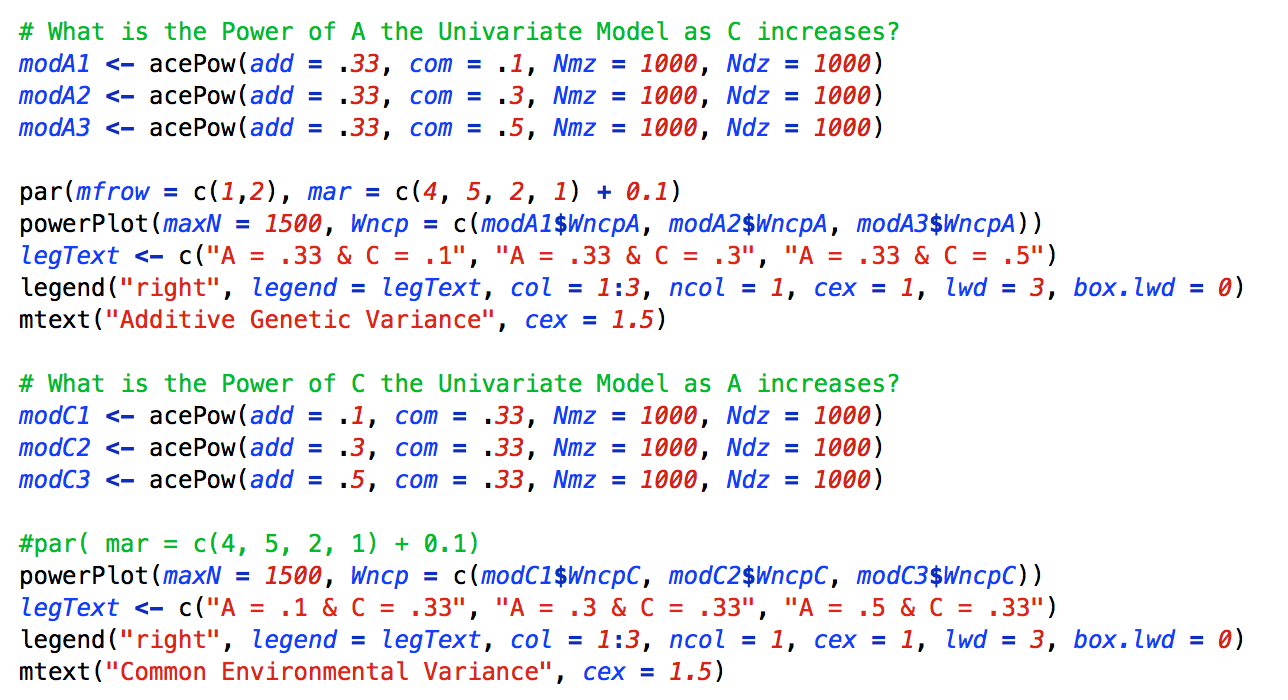
As can be seen, to conduct this power analysis the acePow function was called 6 times and the results were stored in separate R objects: three times for the various A power analyses, and three times for the various C power analyses. Then, to construct the power curve graph, the powerPlot function is called twice. The powerplot function utilizes the Wcnp parameters from the acePow objects, as well as various base R plotting functions such as par and legend.
The figure below presents a graphical depiction the results of the power analysis. As can be seen, the power to detect both variance components depend on the level of the other variance component. As the opposing variance component increases, the power to detect the variance component of interest increases. This is due to the fact that as the standardized variance components of both A and C increase, the standardized variance component of E necessarily decreases and the correlation between the twins (both DZ and MZ) increases. Interestingly, the increase is not symmetrical across A and C. The increase in power is much larger for the A as C increases, than it is for C as A increases. Accordingly, when conducting power analyses, it is essential to consider not only the level of A but also the level of C.
In addition to the power curves, the powerPlot function also produces a table of sample sizes necessary to achieve .2, .5 and .8 power. The power tables for this example are below:
| N1 | N2 | N3 | |
|---|---|---|---|
| .2 | 61 | 33 | 11 |
| .5 | 272 | 148 | 47 |
| .8 | 623 | 338 | 108 |
| N1 | N2 | N3 | |
|---|---|---|---|
| .2 | 41 | 32 | 24 |
| .5 | 180 | 140 | 104 |
| .8 | 412 | 320 | 238 |
Note that the sample sizes presented in the row for 80% power correspond with the vertical grey dashed lines in the plots.
The second demonstration examines the power to detect the A and C variance components when the ratio of MZ to DZ sample size varied. The ratio of MZ to DZ twins was varied from 5:1 to 1:1 to 1:5. While these ratios are extreme, they illustrate the impact of differential MZ to DZ sample size ratios. The code to conduct the analysis is presented below:
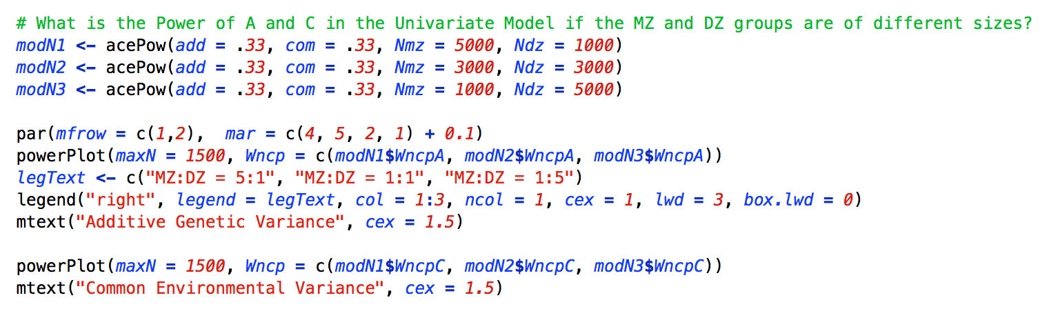
In this example, the variance components remain fixed across all of the power analyses, but the sample sizes for the Nmz, and Ndz arguments vary. Importantly, the powerPlot function is essentially unchanged from the previous example.
As can be seen in the left panel of the figure below, to interpret the power analysis, the power to detect A is maximized when there are approximately equal numbers of MZ and DZ twins. Deviations from a 1:1 ratio in either the MZ or DZ direction, reduce the power to detect a significant A component. By contrast, the power to detect C is highest if there are a surplus of DZ relative to MZ twins, but the increase in power is minimally better than an equal MZ:DZ ratio. A surplus of MZ twins is strongly reduces the power to detect C.
The third demonstration examines the power to detect a significant A variance component for continuous data relative to binary data with prevalences ranging from .5 to .05. For this example we kept the A and C variance components at .33 and used equal numbers of MZ and DZ twins. As can be seen in the Figure below, there is a large reduction in power for a median split (prevalence = .50) relative to a continuous variable, and as the prevalence of a phenotype decreases, the power to detect A decreases.
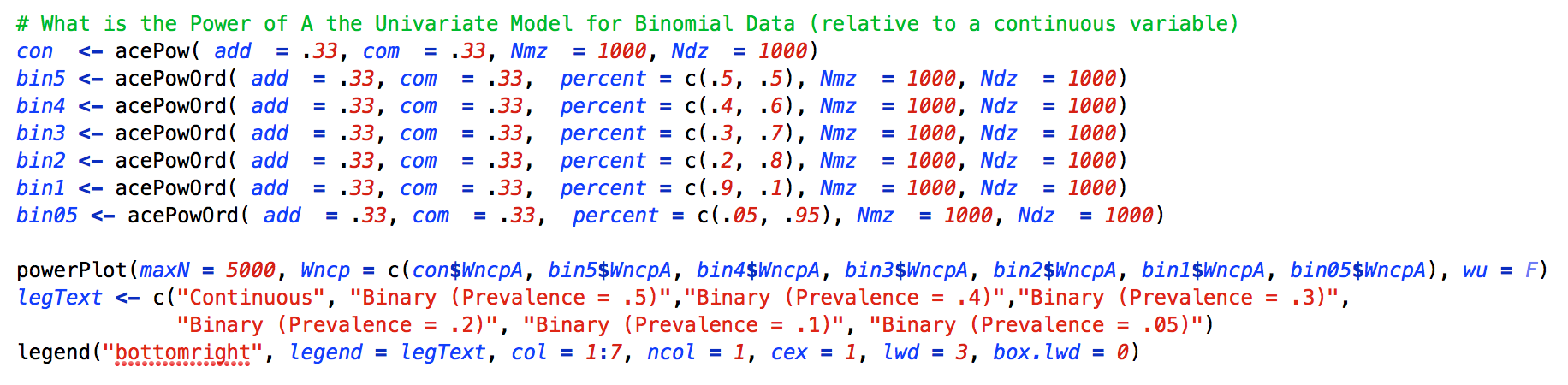
As with the previous examples, the acePowOrd function is run several times, but for this example the key change is in the prevalence. This function requires that the sum of the percent argument is 1, or you will get an error message. For all other intents and purposes, the powerPlot function operates in the same manner as the previous examples.
The next demonstration examines the power to detect a significant genetic correlation (Rg) between two phenotypes. As the power to detect a significant Rg depends on the magnitude of the genetic variance in the phenotypes under examination, the values of A, which are equal across the two phenotypes, were varied from .3 to .4 to .5 and the values of Rg were varied from .1 to .3 to .5. The value of C for both phenotypes was set to .33. and the value of E was adjusted to ensure that the variance of all of the traits was 1. As can be seen, the addition of an additional phenotype makes the specification of the power analysis more complicated. The script to conduct this analysis is presented below:
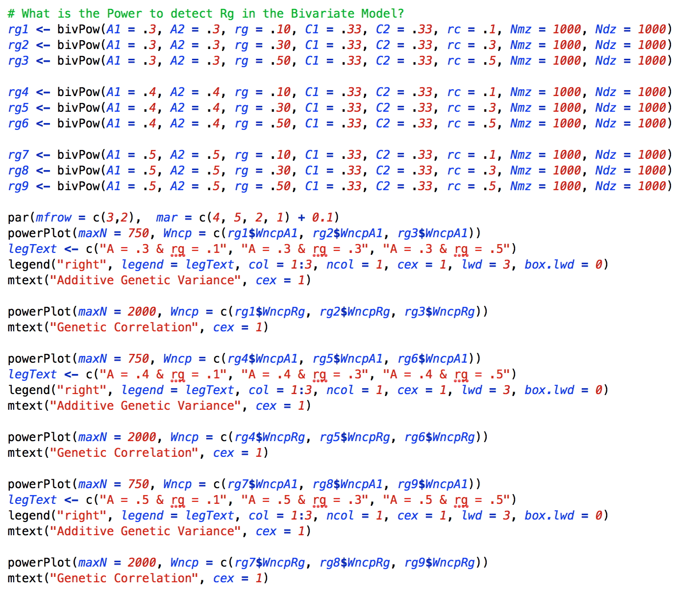
For this example, the bivPow function is run 9 times to capture the various combinations of parameter values that are presented in the power analysis. For simplicity, the continuous bivariate model is run, but if you are interested in using binary/ordinal data for a covariance, the difference between the bivPow and the aceBivPowOrd functions are trivial (the worked example is presented in the full script).
The interpretation of the power analysis depends on all of the parameters in the model. Briefly, the left column of the figure below presents the power curves for the A variance component in the first phenotype. As was the case with the univariate models, as the magnitude of the additive genetic variance component increases, so too does the power to detect it. The right column presents the power curves for Rg. As can be seen, the power to detect significant Rg increases as both the magnitude of Rg increases and as the magnitude of A increases. Importantly, the magnitude of the C variance component (which is not presented here) also affects the power to detect A and the power to detect Rg.
The next demonstration examines the power to detect significant qualitative (different genetic factors) and quantitative (same genetic factors to differing extents) sex limitation models. For this example, the sexLimPower function is run 5 times to test the power to detect qualitative sex limitation and 3 times to detect quantitative sex limitation. The script to conduct this power analysis and plot the power curves is presented below:
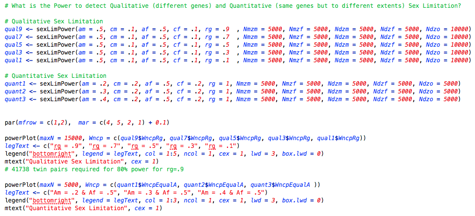
As can be seen in the left panel of the figure below, the power to detect a significant qualitative sex limitation is relatively low compared to the previous models. Specifically, it would take more than 5000 twin families to achieve .8 power to detect a correlation of .5 between male and female genes (am = af = .5, cm = cf = .1). This is a relatively low correlation between the genetic components of a phenotype for males and females. As the genetic correlation between males and females increases (into more reasonable ranges), the power to detect qualitative sex limitation decreases. Because the power to detect qualitative sex limitation depends on the magnitude of the genetic variance in both sexes, as it is easier to detect different genetic factors that affect the phenotype in males relative to females when the magnitude of genetic variance in both sexes is high.
The quantitative sex limitation power curves are presented in the right panel of the figure above. For quantitative sex limitation there are several possible hypotheses that can be tested. The power analysis presented above tests the power to detect a different magnitude of genetic variance in males and females. As can be seen, as the magnitude of genetic variance in males increasingly differs from females, the power to detect this difference increases. Specifically, when the standardized genetic component is .2 in males and .5 in females, 2556 twin pairs would be required to achieve .8 power. Note that for quantitative sex limitation model to make logical sense, the correlation between the genetic factors must be equal to 1 (rg = 1).
The final demonstration illustrates how to conduct a power analysis for a multivariate twin model. For this example, I am going to present a model to test for additive genetic variance in a common pathway twin model but the process can be followed for alternative models. Note that this is a 1 df test of significance. A discussion of multiple df significance testing for variance components is presented in the next section.
Three functions are provided that allow for the simulation of (1) Cholesky decomposition twin data, (2) independent pathway twin data, and (3) common pathway twin data. Because of the complexity of these models, it can be cumbersome to simulate data with the specific nuances that a researcher is interested in, in no small part because there are multiple parameters that must be provided. Furthermore, the list of possible power analyses that could be of interest is quite large. Thus, the method presented below shows users how to conduct the power analysis “manually”.
The function to simulate Cholesky decomposition twin data is:
CholSim( aLower, cLower, eLower, Nmz, Ndz)
The aLower ,cLower, and eLower arguments take lower triangular “Cholesky” matrices, and the Nmz, and Ndz matrices are the number of MZ and DZ families, respectively. These lower triangular matrices can be very difficult to specify, as most people find it more difficult to think in terms of Cholesky matrices and easier to think in terms of correlation matrices. Thus, it is probably more useful to use the bivariate ACE functions above to calculate the power for a specific correlation, rather than to use this function to manually calculate power.
The function to simulate independent pathway twin data is:
indPathSim( aLoad, cLoad, eLoad, specA, specC, specE, Nmz, Ndz)
The aLoad ,cLoad, and eLoad arguments allow the user to specify the factor loadings for each variance component. The specA ,specC, and specE arguments allow the user to specify the residual A, C and E components. The Nmz, and Ndz matrices are the number of MZ and DZ families.
Finally, the function to simulate common pathway twin data is:
comPathSim( aL, cL, eL, load, specA, specC, specE, Nmz, Ndz)
The aL ,cL, and eL arguments allow the user to specify the standardized A, C and E variance components for the latent variable. The load argument allows the user to specify the factor loadings of each item on the latent variable. The specA ,specC, and specE arguments allow the user to specify the residual A, C and E components. The Nmz, and Ndz matrices are the number of MZ and DZ families.
For this demonstration we will calculate the power for the common pathway model. The full script to conduct this power analysis and plot the power curves can be found by clicking on the figure below. The script to simulate the data is presented below:

First, we need to simulate data (which is done using the function above). As can be seen, for this example the latent variable is simulated to have standardized A, C and E variance components of .3, .3 and .4 respective. The factor loadings range sequentially from .9 to .5. and the specific A, C and E variances for each item are specified at .2. Finally, we simulate data for 2000 MZ and 2000 DZ twins (thus the sample size is 4000 in this case).
Second, we need to fit the full and reduced model to calculate the difference in the -2 log likelihood for the full and the reduced models. This can be done using your own common pathway script, the scripts provided from the IBG workshop, or the script provided here. Once the full and reduced models have been run, subtract the -2 loglikelihood of the full model from the -2 loglikelihood of the reduced model and divide the difference by the total number of MZ and DZ families. An example is presented below based on the simulated example above:
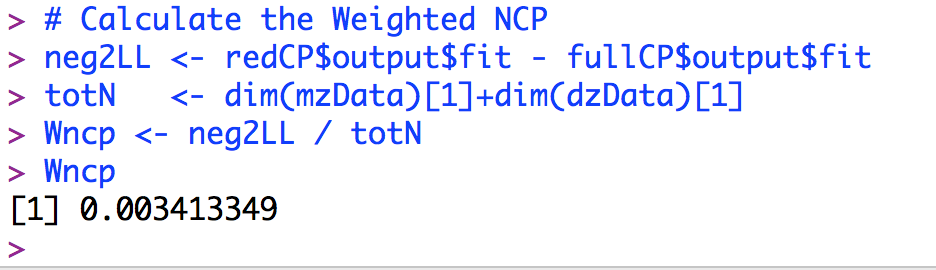
The Wncp value for this example is 0.0034. If we increase the value of the additive genetic variance for the latent variable to A = .3 (with C = .2 and E = .5), the calculated Wcnp parameter is 0.0093. If we again increase the value of the A for the latent variable to A = .4 (with C = .2 and E = .4), the calculated Wcnp parameter is 0.0347. These values can be inserted into the powerPlot() function, as follows:

This will produce the following figure:
As can be seen in the figure, the power to detect A increases as the magnitude of A increases (and the magnitude of E decreases). While this is an obvious result, using this method, it is possible to test for any parameter of interest in the common pathway model.
Post hoc power analyses. The discussion to this point has focused on a priori power analyses (or power analyses conducted before a grant is submitted and data is collected). Another common usage of power analyses is post hoc power analysis, where the values obtained from a specific sample are used to calculate the power to detect a significant effect. While it is possible to insert the obtained values from a completed analysis into the functions provided here, existing data typically has `quirks' that may not be approximated using simulated data. Because it is common practice to run full ACE models and follow them up with reduced AE and CE models, it is quite simple to compute the ncp directly from the observed results. Specifically, the difference in the likelihood for the full and the reduced models (as estimated in the data), can be divided by the observed sample size to obtain the weighted ncp, in the same way as was described above. This weighted ncp can be used to calculate the power for a range of sample sizes.
More elaborate genetic models. The power analysis functions that are presented here cover several common, though basic, scenarios that are routinely encountered in the analysis of twin data. There are numerous alternative models that are not directly covered in these functions, such as common and independent pathway models. There are two primary reasons for not including these functions. First, it is very cumbersome for users to enter the dozens of necessary parameters that are required for these more advanced models. Second, and intimately related, most researchers who estimate these models have specific preferences regarding how the models are parameterized that differ across research groups, while remaining under the same general umbrella. That said, those interested in conducting power analyses for these more advanced models can utilize the same procedure manually (without the use of the simplifying power functions).
Third, and more important, the standard Type I Error rate at α = .05. In twin models in particular, but in any model where there is a strong theoretical boundary on a parameter, the Type I Error rate will be over estimated. Because variances must be positive, the Type I Error rate for a single variance component is actually an equal mixture of a χ2 distribution with 1 df and a χ2 distribution with 0 df. It turns out that for the 1 df case, the solution for the mixture reduces to setting α = .10. For the general multiple df tests, there is no straightforward correction for the Type I Error rate, and therefore must be calculated empirically. Dominicus et al. (2006) provide an analytical solution for the specific case of comparing the full ACE with the E only model (2 df test). Not taking the mixture of χ2 distributions into consideration will under estimate power.