GW-SEM (Genome-Wide Structural Equation Modeling) is a software package designed to estimate Structural Equation Models (SEM) on a genome-wide basis. This tutorial aims to walk users through the process of conducting a Genome-Wide Structural Equation Modelling Analysis using the software package GW-SEM. We have attempted to make the tutorial as user-friendly as possible. To this end, we have provided a series of simulated datasets that allow users to test the features of GW-SEM and better understand the analytical procedure. The files can be viewed (which is particularly instructive for setting up your own data) by clicking on the highlighted portions of the text or figures. Similarly, right-clicking on the same features allows the files to be downloaded.

To run the tutorials, users should create a directory on their computer and save (1) the phenotype file and (2) the genotype file. Users must then open R, load OpenMx, and the GW-SEM functions. The steps to obtain the required software are described in the next section.

GW-SEM is a free, open source software program that relies on other free, open source software programs that can be downloaded by following the links in this section. The software provides specific functions to estimate four common SEMs: a one-factor model, a one-factor residuals model, a two factor model, and a latent growth model (LGM). GW-SEM utilizes the R computing environment, allowing users to capitalize on its inherent benefits. R can be downloaded by clicking on the R icon and following the appropriate links for your specific computer.

To fit the SEMs, GW-SEM uses OpenMx, an open-source software package that fits a variety of advanced multivariate statistical models. You can learn more about OpenMx by clicking on the OpenMx Guinea pig. To install OpenMx, open the R console and paste the following code in the terminal window:

source('http://openmx.psyc.virginia.edu/getOpenMx.R')

Alternatively, OpenMx can be downloaded from CRAN, although that version lacks parallel computation features on some platforms. A supplementary goal of GW-SEM is to create a set of functions for easy use by researchers who are not dedicated data analysts. The tutorial below is designed to clarify the analytical process. Most users will likely apply only the preprogrammed functions. Advanced users could edit the functions to create other structural equation models.

The GW-SEM functions are presented here. If you right click on the icon, you can save the file to a local folder.

The first step in conducting the GWAS is setting up the data. To run any of the GW-SEM functions, you must have two separate files: the phenotype file and the SNP file. In both files, the data for each subject are stored by row and the columns represent the items and covariates (in the phenotype file) and SNPs in the SNP file. The subjects (rows) in both files must match (i.e., the same person must be on the same line in both files). An example of a phenotype file is presented above (after being loaded into R), and an example of the first 10 columns of a SNP file is presented below. As genotype files can be very large, you will not want to load the whole file into R.

WARNING: GW-SEM does not conduct any data cleaning or quality control (QC) steps, which are essential for appropriate genomic analyses. Both the phenotype and genotype file should be properly QC'd prior to analysis. Here are a few links to get you started with QC: 1, 2, 3). GW-SEM can analyze both “Hard Call” and “dosage” genotype files. All missing values must be coded NA (which is the default code for missing data in R).

The analytical routine for each GW-SEM function follows three general steps:

1. Calculate the SNP-invariant covariances.
2. Calculate the SNP-dependent covariances.
3. Fit the SEM.

Each of the step is discussed in detail below

To conduct GW-SEM, it is necessary to compute the covariances between all of the variables that are analyzed in each model. Because most of the variables do not change depending on which SNP is being analysed, these covariances can be computed once and used in every model. Because all of the item-item, item-covariate and covariate-covariate covariances (and variances) do not depend on which SNP is being tested, we label them SNP-invariant covariances.

The SNP-invariant covariances are calculated using the facCov() function:

facCov( dataset, VarNames, covariates)

where dataset is a dataframe in R, VarNames is a list of the variable names of the items, and covariates is a list of covariates. The function returns covariances, weights, and standard errors of all of the variances, covariances, means and thresholds for all of the items and covariates.

Because this function runs quickly (even for a relatively large number of items), the function is called directly by the other functions. Therefore users do not actually need to call this function to conduct the GW-SEM. This function is useful to ensure that the data are properly organized and there are no peculiarities with any of the variables they plan on including in their analyses.

The second step in the analysis is to estimate the SNP-dependent covariances. These calculations are conducted using the snpCovs() function:

snpCovs( FacModelData, vars, covariates, SNPdata, output, zeroOne, runs, inc, start)

• FacModelData the file path to the text file (outside R) with the items and covariates data.
• vars a list of items to be included in the analysis (from FacModelData).
• covariates a list of covariates to be included in the analysis (from FacModelData).
• SNPdata the file path to the text file with the SNP values (outside R).
• output the prefix for the output files created during this step (covariance, standard errors and weights).
• zeroOne a logical (TRUE or FALSE) statement regarding whether to use the Mehta, Neale & Flay (2004) approach to obtain means and variances from ordinal data.
• runs the number of batches of SNPs to be analyzed.
• inc the number of SNPs included in each batch.
• start the column in the SNP file of the first SNP to be sampled.

To demonstrate how to use this function, we use simulated data for a one factor model with 5,000 observations and 10,000 SNPs. A schematic representation of the one factor GW-SEM model is present on the right. In the Figure, the latent factor (F₁) causes the observed items (x_k). The association between the latent factor and the observed indicators are estimated by the factor loadings (λ_k). The residual variances (δ_k) indicate the variance in (x_k) that is not shared with the latent factor. The regression of the latent factor on the SNP (for all SNPs in the analysis) is depicted by (β_k). It is important to mention that in order for a one factor model to be identified, you will need at least three items, but more items will improve the measurement components of the latent variable. While there are statistical tricks to that can be used to identify latent variables with two indicators, GW-SEM does not incorporate these tricks. The phenotype data and SNP data for the example can be downloaded by clicking here [Phenotype file] [SNP file]. The files should be saved in the same directory. The code to calculate the correlation between the SNPs and the items/covariates is presented below.

snpCovs( FacModelData = "Ord1fac.txt", vars = c("i1","i2","i3","i4","i5"), covariates = c("c1","c2","c3"), SNPdata = "SNP.txt", output = "Ord1fac") zeroOne = FALSE)

While the arguments are not included in the current demonstration, the runs and inc options are very useful in the testing phase, as they allow the user to conduct a limited analysis in a relatively short time. For example if you wanted to make sure that the analysis is set up properly, you may want to run 300 SNPs in three batches. Thus, she would set runs = 3 and inc = 100. Further, the start argument is very useful if the function was to stop for some reason (e.g., the cluster on which you are running the analysis was shut down for some reason in the middle of the analysis, or your computer restarted). To find the column to restart, you can generally look last SNP that was analyzed and start at the next one.

The output from snpCovs() is saved in three separate files (outside of R) as specified by the output argument: the covariances are saved in Ord1faccov.txt, the weights are saved in Ord1facwei.txt,and the standard errors are saved in Ord1facse.txt. Each file is organized so that each row is the covariance/weight/standard error of the SNPs and each column is an item/covariate.

This step effectively calculates a GWAS for each item/covariate. The covariances and the weights are passed to the next function, but the covariances and the standard errors can be very useful in trouble shooting (e.g., for finding covariances or standard errors that are inappropriately large, small, or inconsistent with your expectations).

The final step in GW-SEM procedure fits one of the SEMs. To continue the example from above, we use the same data. The function to fit the one factor SEM is gwasDWLS():

gwasDWLS( itemData, snpCov, snpWei, VarNames, covariates, runs, output, inc )

• itemData the path to the text file (outside R) with the item and covariates.
• snpCov the path to the text file (outside R) with covariances between the SNPs and the items/covariates.
• snpWei the path to the text file (outside R) with the weights.
• VarNames the list of items.
• covariates the list of covariates.
• runs the number of batches of SNPs to be analyzed.
• output the file name for the output file.
• inc the number of SNPs included in each batch.

Using the output from the snpCovs() function as input for the gwasDWLS() the code to fit the one factor SEM to the data is:

gwasDWLS( itemData = "Ord1fac.txt", snpCov = "Ord1faccov.txt", snpWei = "Ord1facwei.txt", VarNames = c("i1","i2","i3","i4","i5"), covariates = c("c1","c2","c3"), output = "Ord1Facout.txt")

Again, the runs and inc options can be used to conduct a limited analysis on a subset of the SNPs.

The output from gwasDWLS() is saved in the file specified by the output argument. In the current case it is saved in "Ord1Facout.txt" This file is smaller than the genotype file and can be read into R to examine the results or create tables and figures for publication. The first 6 lines fo the output file are presented below.

There are many ways to present the results of genome-wide association analyses. A common approach is to construct two summary figures. The first is a Manhattan plot, which plots the -log₁₀ p-values on the y-axis against the base-pair position of the genome on the x-axis. Because Linkage-Disequilibrium (LD) creates a correlation structure for the SNPs (with proximate SNPs being more correlated), adjacent p-values tend to be similar so that the plots tend to resemble the Manhattan skyline. This pattern does not appear with simulated data that do have not incorporated LD structure into the simulation, as is shown here. Many R functions for Manhattan plots can be found via Google search. Here we make a simple one using the basic plot() function in R. Using the one factor GW-SEM example above, the following code:

creates a plot that looks like this:

The red line in the figure denotes genome-wide significance (p<5×10^-8) and the blue line denotes suggestive significance (p<1×10^-5). Note that most of the dots in the figure (that denote the significance for that specific SNP) fall well below the blue line. There are five SNPs that are above the blue line (which about what you would expect by chance), and one SNP that is approximately one the red line. Most researchers carefully examine each of the SNPs above the suggestive significance threshold, while keeping in mind that these SNPs do not reach the standard for genome wide significance.

To identify the SNPs with the highest levels of significance, it is possible to sort the SNPs by the p-values threshold with:

This will produce the following in the console window:

As you can see, rs8214 is the most significant SNP, but it just misses the genome-wide significance threshold. (This SNP was simulated to have a real effect on the phenotype.)

The second plot that researchers typically examine is the QQ plot. QQ plots compare the theoretical quantiles of test statistics (such as t or Z scores) with the observed quantiles (or the test statistics that you got from your GWAS with a the expected test statistics if the null hypothesis was true). While QQ plots can be obtained using the basic stats package in R, the car package (written by John Fox) makes much nicer graphs and is very user friendly. The code to make a QQ plot using the car package is:

This will produce the following QQ plot:

As you can see, there is very little inflation in the test statistics relative to the null in this example, which is to be expected since the data were generated under the null hypothesis.

The final step in the process is to examine the model's parameter estimates, and in particular the factor loadings. The estimates of all the parameters for each of the SNP loci are stored in "estimates.txt". Because the model for each SNP is slightly different, the regression of the factor on the SNP may subtly change the parameter estimates for each locus. Overwhelmingly, these changes will be negligible as the SNPs are not expected to account for a large proportion of the variance in the latent factor, but it is essential to examine the parameters to report the findings. Aside from the regression of the SNP on the latent factor, the most interesting parameters are the factor loadings. The first six factor loadings can be seen below (after being read into R), as well as the loadings for the suggestively significant SNP, rs8214.

As can be seen, the values for the factor loadings change minimally with each SNP. Even when the SNP is almost genome wide significant, the change in the factor loadings is only at the 3^rd decimal place. If, however, the factor loadings are wildly different for a specific SNP, it is likely that there was some problem with the model optimization. Any subsequent interpretations of the model at such a locus should be treated with extreme caution and skepticism. If these data were real, and we wanted to write up the results for publication, we would typically take all of the parameter estimates and put them into a path diagram (similar to the one earlier in this section) with the appropriate parameters on the appropriate path. All of the parameter estimates for rs8214 are shown at the bottom of the figure above. The first set of parameters are the regressions of the items on the covariates (c1_1 is the regression of item 1 on covariate 1). Next is the regression of the latent factor on the SNP (snp), followed by the loadings (l1 is the factor loading for the first item). Then we have the variances (var_c1 is the variance of the first covariate and SNPvar is the variance of the SNP). Finally we present the means (with mean_c1 being the mean of the first covariate). Note that there are no item means and variances because this example uses ordinal data where the means and variances of the items are fixed and the thresholds are estimated.

At this point, you may want to refer to the UCSC Genome Browser, NCBI dbSNP, and LocusZoom (among various post-analysis processing steps) to find additional information about the significantly associated SNP.

To summarize, to conduct a one factor GWAS, all you need is two lines of code. For the example presented here those two lines are:

snpCovs( FacModelData = "Ord1fac.txt", vars = c("i1","i2","i3","i4","i5"), covariates = c("c1","c2","c3"), SNPdata = "SNP.txt", output = "Ord1fac") zeroOne = FALSE)

gwasDWLS( itemData = "Ord1fac.txt", snpCov = "Ord1faccov.txt", snpWei = "Ord1facwei.txt", VarNames = c("i1","i2","i3","i4","i5"), covariates = c("c1","c2","c3"), output = "Ord1Facout.txt")

The R Script to run this tutorial is presented here.

The next SEM included in the GW-SEM package is the residuals model. The Figure on the right presents a schematic representation of the residuals model, which has very similar parameters to the one factor model presented above. Importantly, the same identification requirements are the same as the one factor GW-SEM model above. The notable difference is that the individual items are regressed on each SNP (γ_k). The residuals model allows researchers to regress a SNP on the residuals of the items that contribute to a latent factor. It is also possible to fit the residuals model so that the latent factor and a subset of the items are regressed on the SNPs. If you do this, in order to identify the SEM it is only possible to regress a subset of the items and the latent factor on the SNP or the model will not be identified. The model is still identified if all of the item residuals are regressed on the SNPs, but the latent factor is not. The syntax to fit the residuals model is:

snpCovs( FacModelData, vars, covariates, SNPdata, output, zeroOne, runs, inc, start )

resDWLS( itemData, snpCov, snpWei, VarNames, covariates, resids, factor, runs, output, inc)

The snpCovs() function is exactly the same function as was used for the one factor GW-SEM and the resDWLS() is very similar. The only two arguments that differ from the single factor model are resids which is a list of the items to be regressed on the SNPs, and factor which is a logical value asking whether the latent factor is to be regressed on the SNPs. The other arguments operate in exactly the same way as with gwasDWLS(). This similarity makes it easy to conduct follow-up analyses for the one factor model with minimal additional steps.

SNP data and Phenotype data for the demonstration of the residuals model should be saved into a file folder along with the the GW-SEM script.

We will now walk through an example of using the residuals model. For the example presented here we will compare the results from a one factor GW-SEM model to the residuals GW-SEM model. This means that in addition to estimating the residuals model we will also estimate the one factor model. If you do not wish to estimate the one factor model, gwasDWLS() command can be removed. The code for the example analysis that we conducted is presented below.

snpCovs( FacModelData = "Ord1fac.txt", vars = c("i1","i2","i3","i4","i5"), covariates = c("c1","c2","c3"), SNPdata = "SNP.txt", output = "Ord1fac") zeroOne = FALSE)

gwasDWLS( itemData = "Ord1fac.txt", snpCov = "Ord1faccov.txt", snpWei = "Ord1facwei.txt", VarNames = c("i1","i2","i3","i4","i5"), covariates = c("c1","c2","c3"), output = "Ord1Facout.txt")

resDWLS( itemData = "Ord1fac.txt", snpCov = "Ord1faccov.txt", snpWei = "Ord1facwei.txt", VarNames = c("i1","i2","i3","i4","i5"), covariates = c("c1","c2","c3"), resids = c("i1","i2","i3","i4","i5"), output = "OrdResOut.txt")

The output from gwasDWLS() is saved in "Ord1Facout.txt" and the output from resDWLS() is saved in "OrdResOut.txt" The first 6 lines of each output file (after being read into R) are presented below.

As can be seen, the output from the residuals model is a little more more complicated, with a regression coefficient, standard error, t statistic and p-value associated with each of the items. As with the one factor GW-SEM, to summarize the output it is useful to construct Manhattan plots of the p values for each item. To have a point of comparison, we will first construct a Manhattan plot for the one factor model.

The Manhattan plot for the one factor GW-SEM can be constructed in the same way as was done above (in fact, because we have used the same labels for the items and the covariates even though the actual data differ, it is possible to use exactly the same code). The one factor GW-SEM Manhattan plot for the current example is presented below.

Now let's put together the Manhattan plot for the 5 items. The code to do this is presented below. To stack the plots on top of each other the mfrow argument of the par() function is used, and to adjust the spacing around the plots the mar option is used.

The resulting set of Manhattan plots is presented below.

As can be see in the Manhattan plot of the one factor GW-SEM analysis, there is a genome-wide significant association somewhere in the middle of the set of SNPs. Interestingly, there are absolutely no significant, or even suggestive, associations for the for any of the residuals.

Now, let's compare the top hit from the one factor GW-SEM to the residuals GW-SEM by searching for the genome-wide significant SNP from the one factor GW-SEM and selecting only that SNP from the residuals model. The code to do this is presented below.

The resulting output is:

As can be seen, the most significant association is between the latent factor and rs5218. Looking specifically at rs5218 in the residuals output shows that there is a consistent relationship between the SNP and all of the items. Specifically, the β’s ≈ .10 for all of the items, while the β = .18 for the latent factor. Further, the p-values for the items range from ≈ .01 to .001, falling well below even the suggestive threshold for genome wide significance. Accordingly, if we were to run a GWAS on each item separately we would conclude that there is no association between any of the items and any of the SNPs, but with the one Factor GW-SEM a genome-wide significant association can be detected. This is the pattern of results that we would expect if the SNP was associated with the latent factor rather than one of the specific items. By contrast, if the SNP was associated with one of the items but not the latent fator, then we would observe a single peak for that item, and a very reduced, likely non-significant peak for the latent factor (partly as a function of the magnitude of the significant item's factor loading).

As with the one factor GW-SEM, it is important to look at the other parameters in the model. For the residuals model, the parameters are stored in "resEstimates.txt" and for the one factor model they are stored in "estimates.txt". Rather than looking at the first several estimates, this time we will look at the estimates for rs5218 (the significant SNP in the one factor model) in both the residuals model and the one factor model. These estimates are presented below.

In the above figure, the estimates of the corresponding parameters are very similar. In fact, if the estimates were rounded to two decimal places (as is common in most publications), they would appear equivalent.

Finally, it is possible to construct a QQ plot of the test statistics. Because five items are regressed on the SNP in the residuals model, it is advisable to construct 5 QQ plots in addition to the QQ plot for the one factor model. The code to conduct these plots is presented below.

The produces the subsequent plots.

For the current example, there is no serious inflation of the test statistics relative to what would be expected under the null hypothesis.

A script to run all of the analyses for the residuals model can be found here.

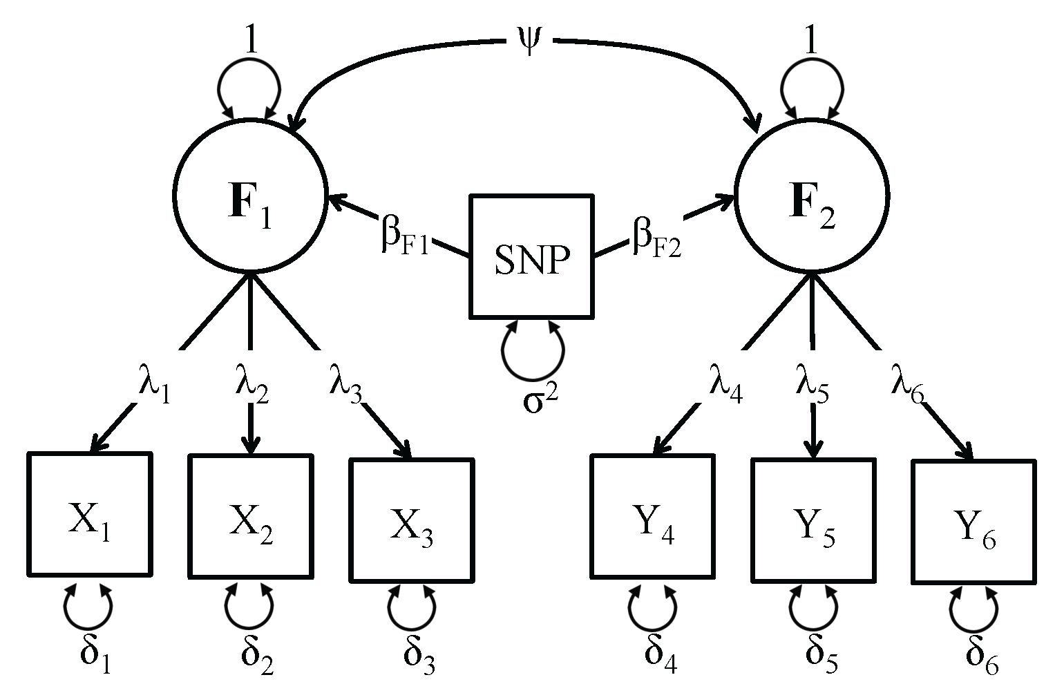The third SEM included in the GW-SEM package is the two factor SEM. The Figure on the right presents a schematic representation of the two factor model. In this model, both latent factors (F₁ & F₂) are regressed on every SNP (β_F1 & β_F2) and the latent factors are allowed to correlate (ψ). It is important to note that in order for the two factor SEM to be identified, both latent factors must have at least three indicators (just as the one factor SEM had to have three indicators for the latent factor). While it is possible to include cross-loadings (items that load on both factors), it is necessary to have at least one unique item per factor. The syntax to fit the two factor model is:

snpCovs( FacModelData, vars, covariates, SNPdata, output, zeroOne, runs, inc, start )
twofacDWLS( itemData, snpCov, snpWei, f1Names, f2Names, covariates, runs, output, inc)

Again, the snpCovs() function is the same function as was used for the one factor GW-SEM, but for the two factor model, a list of all of the items for both factors are included in the vars option. The twofacDWLS() is very similar, with two arguments that differ from the single factor model: f1Names which is a list of the items that are indicators of Factor 1, and f2Names which is a list of the items that are indicators of Factor 2. The other arguments operate in exactly the same way as with gwasDWLS().

Just as was done for the previous examples, the SNP data and the Phenotype data for the demonstration of the two factor model should be saved into a file folder along with the the GW-SEM script.

As an example, we will fit the two factor model by running the two lines of code presented below.

snpCovs( FacModelData = "Ord1fac.txt", vars = c("y1","y2","y3","y4","x1","x2","x3","x4"), covariates = c("c1","c2","c3"), SNPdata = "SNP.txt", output = "Ord2fac") zeroOne = FALSE)

twofacDWLS( itemData = "Ord2fac.txt", snpCov = "Ord2faccov.txt", snpWei = "Ord2facwei.txt", f1Names = c("y1","y2","y3","y4"), f2Names = c("x1","x2","x3","x4"), covariates = c("c1","c2","c3"), output = "Ord2FacOut.txt")

The output from twofacDWLS() is saved in "Ord2FacOut.txt". The first few lines of the output file (after being read into R) are presented below.

As can be seen, the two factor GW-SEM results present a regression coefficient, standard error, t-statistic and p-value associated with each factor. As with the one factor GW-SEM, it is useful to construct manhattan plots for the p-values for each item. The Manhattan plot for the two factor GW-SEM can be constructed in an analogous way as the residuals GW-SEM above. The code for the two factor GW-SEM Manhattan plot is presented below.

The resulting Manhattan plot is:

Looking at the Manhattan plots, it appears that there are two hits for each factor. To dig deeper into these associations, we can examine the top set of SNPs for both Factors, as shown below. For simplicity, we will only look at the regression coefficients, the standard errors and the p-values for each factor.

The first set of results sorts the p-values with respect to Factor 1. As we saw on the Manhattan plots there are two genome-wide significant associations for Factor 1. The top hit for Factor 1 is rs2178 and the second hit is rs6001. Looking at the p-values, it is clear that that rs2178 is only associated with Factor 1, as the p-value for the association with Factor 2 is p = .67. The second set of results sorts the p-values with respect to Factor 2. Again there are two significant hits: rs2014 and rs6001. Similar to the Factor 1 case, rs2014 is only associated with Factor 2 (the p-value for its association with Factor 1 is .99). Importantly, rs6001 is associated with both factors. Accordingly, for this example there are SNPs with significant associations: rs2178 is only associated with Factor 1, rs2014 is only associated with Factor 2, and rs6001 is associated with both Factor 1 and Factor 2.

As with the previous models, it is now time to look at the other parameters in the model. For the two factor model, the parameters are stored in "twoFacEstimates.txt". Rather than looking at the first several estimates, this time we will look at the estimates for rs2178, rs2014, and rs6001 (the significant SNPs in the two factor model). These estimates are presented below.

The estimates of the corresponding parameters are very similar for each of the three significant SNPs. As would be expected, the largest difference between these models is that for the rs6001 model, the factor correlation is notably (but subtly) smaller than for the other two models (as shown in the cov12 column of the output), suggesting that the pleiotropic genetic effects are responsible for a part of the association between these latent factors.

Finally, will construct a QQ plot for each factor. The code to conduct these plots is presented below.

The produces the subsequent plots.

For the current example, there is no serious inflation of the test statistics relative to what would be expected under the null hypothesis. Note the two points that are substantially above the line in the top right corners of both QQ plots. These denote the significant SNPs for both factors.

A script to run all of the analyses for the residuals model can be found here.

The fourth and final model included in GW-SEM is the Latent Growth Model (LGM). The Figure on the right presents a schematic depiction of the latent growth model, where the factor loadings are fixed to specified values, and the means (μ_F), variances and covariances (Ψ) of the latent growth parameters are estimated. Each latent growth factor is then regressed on each SNP (β_C, β_L, & β_Q). The Figure presents the quadratic LGM, rather than the linear LGM (note the addition of the third latent growth factor). If you does not wish to fit the quadratic LGM, the function below provides an option for removing it. The Figure presents the standard factor loadings, where the loadings for the latent intercept are fixed at 1, the loadings of the latent linear factor increase from 0 to the number of measurement occasions, and the loadings for the latent quadratic factor are simply the square of the linear loadings. In many cases, this coding will inflate the correlations between the latent growth factors. To prevent this inflation, it is possible to use orthogonal contrasts rather than the standard loadings. The function below provides an option to construct these contrasts automatically. The general syntax for the LGM GW-SEM is:

snpCovs( FacModelData, vars, covariates, SNPdata, output, zeroOne, runs, inc, start )
growDWLS( itemData, snpCov, snpWei, VarNames, covariates, quadratic, orthogonal, runs, output, inc)

For the LGM, the zeroOne argument of the snpCovs function is set to TRUE for ordinal data. By changing this option, the first and second thresholds of the ordinal data are fixed at 0 and 1, respectively, freeing up parameters to estimate the mean and the variance following the Liability-Threshold Model as described by Mehta, Neale and Flay (2004). As the LGM is particularly focused on mean and variance changes, this is an important feature of the covariance model. The only change in the growDWLS() function from the gwasDWLS() function is the inclusion of the quadratic and orthogonal arguments. The quadratic argument is a logical value asking whether to include a latent quadratic growth parameter. The orthogonal argument is a logical value asking whether to use the standard growth loadings or orthogonal contrasts. The code to conduct the LGM GW-SEM is:

snpCovs( FacModelData = "OrdGrow.txt", vars = c("t1", "t2", "t3", "t4", "t5"), covariates = c("c1","c2","c3"), SNPdata = "SNP.txt", output = "OrdGrow") zeroOne = TRUE)

growDWLS( itemData = "OrdGrow.txt", snpCov = "OrdGrowcov.txt", snpWei = "OrdGrowwei.txt", VarNames = c("t1", "t2", "t3", "t4", "t5"), covariates = c("c1","c2","c3"), quadratic = TRUE, orthogonal = TRUE, output = "OrdGrowOut.txt")

The output from growDWLS() is saved in "OrdGrowOut.txt". The first 6 lines of the output file (after being read into R) are presented below.

Similar to the other GW-SEM functions, the LGM GW-SEM results present a regression coefficient, standard error, t-statistic and p-value for each each latent growth factor: the intercept, the linear slope, and the quadratic slope if estimated. Below, we will construct manhattan plots for the p values for each latent growth factor in an analogous way as the residuals GW-SEM above. The code for the LGM GW-SEM Manhattan plot is presented below.

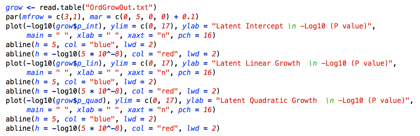
The resulting Manhattan plot is:

Upon inspection of the Manhattan plots, there are three hits for the latent intercept, one hit for the latent linear slope and one hit for the latent quadratic slope. To examine these associations, we can again look at the top set of SNPs for each factor, as shown below. For simplicity, we will only look at the regression coefficients, the standard errors and the p-values for each factor.

The results results for the latent intercept are presented first, followed by the latent linear growth factor, and finally the latent quadratic growth factor. The results are sorted by the p-values with respect to appropriate Factor. As we saw on the Manhattan plots there are three genome-wide significant associations for the latent intercept: rs1529, rs3536, and rs2638. To interpret these effects we would conclude that rs1529 and rs3536 are associated with higher average levels of the trait, regardless of change over time (the direction of the relationship is based upon the sign of the regression coefficient). The second set of results sorts the p-values with respect to latent linear growth factor. The significant association for this factor is with rs3118. Here we would conclude that increasing copies of the SNP increase the rate of growth in the trait over time. Finally, the significant association with the quadratic growth factor is with rs4592. This suggests that increasing copies of the SNP accelerate the quadratic growth of the phenotype. Looking at the p-values, it is clear that that significant associations are factor specific - the SNP associated with one factor has virtually no association with the other factors - as the p-values for the associations with the other factors are greater than the suggestive levels of significance.

As with the previous models, we now turn to the other parameters in the model. For the LGM, the parameters are stored in "growEstimates.txt". Again, we will focus on the estimates for the models with the three significant SNPs rather than looking at the estimates more broadly (rs1529, rs3536, rs2638, rs3118, and rs4592). These estimates are presented below.

The estimates of the corresponding parameters are very similar for each of the significant SNPs. Several of the parameters from the LGM model are the same as those from the previous models, but some of them are slightly different. One of the interesting features of the LGM is that it focuses on the means, variances and covariances of the latent growth factors (the means and variances of the latent traits in all of the previous models were assumed to be zero and one, respectively). The means of the latent growth parameters are presented in the int_mu, lin_mu, and quad_mu columns for the intercept, linear and quadratic growth factors, respectively. Note that these parameters do not change as a function of the SNP that is included. The variances of the latent growth parameters are presented in the v_int, v_lin and v_quad columns for the intercept, linear and quadratic growth factors, respectively. Here the variances of the latent growth factors do change subtly with the inclusion of a significantly associated SNP. The covariances between the latent growth parameters are presented in the i_l, i_q, and l_q columns for the intercept-linear, intercept-quadratic and linear-quadratic growth parameters respectively.

Finally, will construct a QQ plot for each latent growth factor. The code to conduct these plots is presented below.

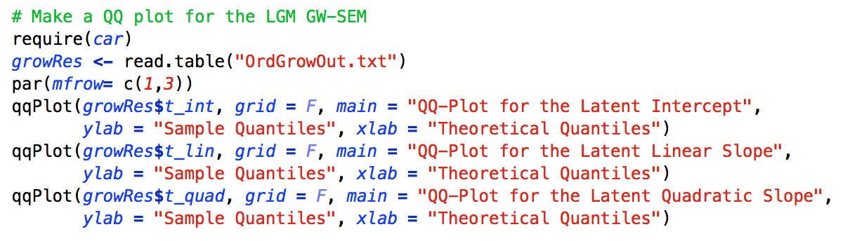
The produces the subsequent plots.

Again, for the current example, there is no serious inflation of the test statistics relative to what would be expected under the null hypothesis. Note the two points that are substantially above the line in the top right corners of both QQ plots. These denote the significant SNPs for both factors.

A script to run all of the analyses for the residuals model can be found here.