SPECT
Image Acquisition And Reconstruction
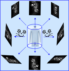
- A Single Photon Emission Computerized Tomography (SPECT) employs 3-D imaging and allows us to evaluate data from a volumetric standpoint
- Acquisition requires that data being collected in a 360 degree axis around the patient (cardiac being the exception)
- Many factors influence the quality of this process and include (not limited to): collimation, acquisition per slice, (sum of the arrays), amount of slices acquired around the circle, distance from the patient, count density, and body attenuation. Can you think of others?
- Once the data has been collected raw data in the form of a cine is usually displayed- this critical step evaluate the acquired data
- Acquiring data represents (a statistical sample) the distribution of radioactive within a cylindrical space/ three dimensional space/volume
- The data can then reconstructed and evaluate different planes within this acquired space - what I refer to as slicing and dicing. The three different reconstructed angles are: transverse, coronal, and sagittal.
- One of the primary methods of image reconstruction Is filtered (convoluted) Backprojection (FBP) - but first we must start with UBP unfiltered Backprojection
- UBP can further be defined as a composite of all the images summed from multi angled, two-dimensional views (sum of the arrays)
- Let us consider a simplistic digital example using the Backprojection concept
- From a planar perspective consider the diagram below. It has a 5 x 5 matrix that contains radioactivity at its center. This displays a hot spot at the center of the image, which we will give a value of 3 representing a certain amount of activity (consider it counts in a pixel)
- When SPECT is applied, multiple angles are taken around the object, hence generating a series of 2D images
- In addition, if we take a series of images 360 degrees around the object the 2-D pixel (cm2), becomes a 3-D voxel (cm3), data acquired for display in the dimensional space
- By the example below, the Anterior Back Projection is the first image (1) which shows an array of hot pixels or data collected in that plane. The collected data shows all pixels in that array having the value of 3. The second image (2) is collected and labeled Lateral Back Projection with the corresponding row showing an array of pixels that contain the same activity. When the image is reconstructed 1 + 2 = 3 the result is the Sum of the Arrays Two Angles Back Projection
- The term Backprojection is used because the images taken are from the perspective of the camera. Hence they are projected back to the camera's point of view. Other way to look at this is the image being acquired is like a movie projection emitting the data onto the surface of the detector. See example
- This simple representation of a SPECT acquisition only shows two images each taken 90 degree from each other. In the real setting there would be between 64 to 128 images acquired around a circle and the matrix size would be either 64 x 64 or 128 x 128
- When the camera stops to acquire an image this is referred to as step or stop
- Notice in the example above, when the images are summed together the streak (background) contains the value of 3 (BKG), however, where the 2 arrays cross each other the value increases to 6, defining the hot spot
- In the real world of imaging, a hot spot within the patient would have created a multitude of streaks with the summed image that would be referred to as a star artifact
- Applying a filtering the reconstruction process will reduce or remove streaks (BKG) leaving the point source visible within the the dimensional space. When this process is used the term FBP is used
- Filter can be used to smooth out noise, remove background, and amplify true counts (more an this later)
- So now let us apply the same concept we just discussed, however, this time the application of a camera is used with a single hot spot in the center
- Our projections are acquired
- The hottest point is in the center in each planar image
- From the four acquired images a transaxial slice is displayed from the summed of the arrays
- The crossing of the two rays define the hot spot
- What happens if we go from 1 to 4 hot spots?
- Depending on the angle of the detector, only a certain number of hot spots can be seen in any of the acquired steps
- Once all images are collected the rays are summed and data can be evaluated in a 3D format
- Notice how different arrays defines the four hot spots - this is an example of UBP
- Reconstruction techniques (summing the images) - Understanding the basic concept
- UBP is the sum of the all the acquired images taken in a 2D format. It is backprojected because of how the camera "sees" the image. If 64 images are collected in a 360-degree rotation, a three dimensional image can be reconstructed by projecting all acquired data back into a circle, as noted in the above example. This new summed image creates a circular volume of data in a 3D matrix
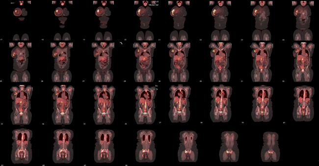
- The end result from these backprojections is the raw data cine being displayed as UBP (L). This image is then reconstructed in FBP and coronal slices are displayed (R).
- If you move your mouse over the FBP images the area is magnified for more detailed analysis
- Moving the arrows on your keyboard will either increase or decrease image magnification
- It should also be noted that while we are talking SPECT the images displayed above are actually PET
******
- Volume data is normally sliced into three different plans as seen above: transverse, sagittal, and coronal
-
- In the computer, the three-dimensional volume of radioactivity representing a function of activity in three-dimensional space. In essence, data can be seen as two-dimensional space: transverse slices stacked, one top of the other, as demonstrated in above
- Furthermore, the technologist can vary the slice thickness by increasing the amount of pixels that makes up the slice thickness
- Since the 2-D pixel becomes a 3-D voxel (cm3)
- In UBP reconstruction, each row of each projected image (consider a row within the matrix) is viewed as a one-dimensional representation of the object's projection. The one-dimensional pixel profiles are modified mathematically, or filtered, and projected back across the two-dimensional slice at their respective angles (ergo Backprojection). Filters are then applied making the image Filtered Backprojection (FBP). Filtering is discussed in detailed ... later.
- Why filter during image reconstruction? The first half of this answer is to eliminate background data, hence remove or filter out the star defect from areas of increased uptake that were acquired. This is demonstrated below
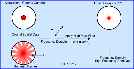
- Gamma camera shows a single hot source in an image (original data) which is taken in planer format
- Now consider the a set of images being taken, of the same object, 360 degrees around this hot spot
- This results of the summed frame image in the spatial domain (UBP) shows a hot area with many rays streaking from it
- If the data is converted to the frequency domain (see Fourier Reconstruction) a profile image would reveal a hot center peak with two smaller peaks on the either side (lower peaks represent the rays). The rays are considered low frequency (LF) background and data that needs to be removed. This LF is also referred as blurring and is discussed below
- Applying a high pass filter during reconstruction removes the majority of the lower frequencies, removing the streaking defect. The final display spatially shows most of the background removed with a center area of activity shows "true" counts
- More on the array and blurring when summing a 3D hot spot
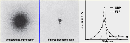
- UBP image (above) shows an large glob of activity, which is a true representation of what is seen when we sum the rays and hot spot. Looking more like a glob than a hot spot
- Issue - the more the stops/slices the greater the size of the hot spot and overlap of data in a 3D image
- The count profile in UBP reveals a formula y = 1/r, where r, at the radius center has the highest count density. The counts anywhere within the count profile is inversely proportional from the distance of the peak activity. This is sometimes referred to as "one-over-r blurring"
- In order to reconstruct this image the blurring must remove the blurring
- As described earlier, to eliminate LF we must apply a high pass filter (example ramp) in the frequency domain that will result in a FBP image
- Why is it necessary to process SPECT in the frequency domain
- Convolution is a mathematical process where 2 functions produce a third function, such is the case in SPECT
- In the spatial domain, (1) is the summed image and (2) is the system blurring
- To remove this blurring, my apply deconvolution, will reveal true counts
- The easiest way to remove blurred counts in the frequency domain
- Fourier reconstruction (converting the spatial domain to the frequency domain)
- Pixels contain data in space that can be converted to frequency space which become a series of sinusoidal curves
- Each pixel is continuous, but has distinctive characteristics representing by the amount of counts in the pixel
- Pixels information is converted into amplitudes and the wave vary by the number of counts in each pixel
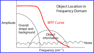
- From the above diagram a MTF curve is displayed along with the location of objects, noise, and background
- The frequency domain
- Conversion into the frequency domain has several characteristics
- The cycles/cm or the amount of oscillations associated with the object's size
- The amplitude defines its height that translates to the amount of counts
- Each pixel represents an amount of counts and pixels in their combination represent a series of objects that may be of different size objects that also determine count densities between the objects being acquired
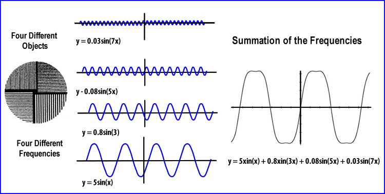
- In another example to help you understand this Objects of a spatial domain, frequency domain, and MTF are compared
A - Represents a series of objects in the spatial domain. As the bars get smaller and darker resolution is lost
B - Is the transformation of the spatial objects into frequencies. Notice how the smaller the bars and relates to the smaller and more cycles/cm. This continues to the point where you can no longer see any oscillations at the same time. Here spatial resolution is lost
C - Shows what the MTF might look like and relates to the ability to see the object and evaluate its frequency
- The last part that fits in this puzzle that fits into our analysis is the Modular Transfer Function - MTF . As you may recall when there is no loss to resolution the MTF's value is 1.0 (100% reproduced). However, just as the you have an increase in cycles per second there will be a corresponding drop in the MTF value. At some point were the reaches zero, data no longer visualized. At that point image noise takes over
- Looking specifically at the MTF note the red line is completely straight. In a hypothetical world this red line would mean that no matter what the size of the object you would be able to see it. Obviously this would never happen, not even in real life ... Tell me, how well can you see that bacteria on your finger?
- In some of the literature you might read there will be a term spatial frequency domain. if you see this, the authors will be referring to the frequency domain, not the spatial domain
- Therefore, different components of the frequency waves mean different things and are composed of the three basic parts: true data, background (lower portion of the wave), noise (higher portion of the wave)/statistical variation and cosmic radiation. From the above image let us interpret what these waves mean.
- The large circle (detector) acquires four objects of different densities and size
- The darker the image the greater amount of counts and the higher its amplitude in a cycle
- The larger the object the wider the wave or the greater the cm of the cycle
- Size variation and the amount of activity is seen spatially and translated into the corresponding frequency
Return to the beginning of the document
Go to the Next Lecture
Return to the Table of Contents
Information and images were acquired through:
- SPECT The Primer, by Bob English
- SPECT in the Year 2000: Basic Principles by MW Groch and WD Erwin
- Determination of Attenuation Maps by H. Zaidi and B. Hazegawa
3/18