Iterative Reconstruction
- Iterative methods (IR) - Is an alternative process to FBP reconstruction that continues to gain popularity in Nuclear Medicine. FBP. The area where IR is currently be utilized the most is in PET, however, its application can be seen in general nuclear medicine SPECT procedures
- This reconstruction method employees the following:
- Attenuation correction map can be employed in the IR process
- Estimation of radiopharmaceutical distribution occurs
- Uniform distribution of activity may be applied or
- Backprojection measurements from an applied matrix can be utilized
- Employs imaging physics
- When compared with FBP there is improved distribution of data, hence quantitative analysis of SPECT data is more accurate
- Since it does not apply the sum of the arrays there is NO star defect
- Iterative methods requires intensive computer processing that is available with current CPU technology. Years ago iterative reconstruction was not practical because CPU processors were too slow
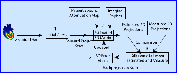
- The following example is a "simple explanation" of the Iterative reconstruction process. Note that the diagram is numbered to match the explanation below
- Data is acquired in a set of 2D matrices (camera stops)180 or 360 degrees around the patient
- Prior to IR the original matrix maybe filtered (smoothed) to reduces statistical noise
- (1) The Initial Guess comes from
- The expected biodistribution of the radio-tracer
- This may be obtained from one of several methods: (a) assume a uniform distribution of activity or (2) apply data from all the 2D backprojection images
- (2) A forward projection step then generates an Estimated 3D Matrix which is influenced by the patient's attenuation map and extra data usually specific to imaging physics
- (3) Then all 2D Estimated Projections are compared to the 2D Measured Projections and are variation identified
- (4) This generates a 3D Error Matrix which then updates step 2 (estimated 3D matrix)
- (2) Estimated 3D Matrix is modified creating a new Estimated 3D Matrix
- The cycle then starts over again hence the term iterative
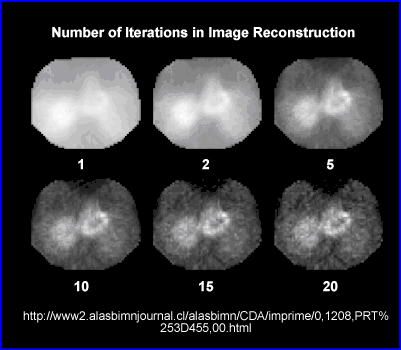
- The user defines the amount of iterations necessary to complete image reconstruction
- Each iteration brings a "truer" count to each voxel
- In the end, the estimated 3D matrix should closely match the "true count" distribution in the 3D structure
- Here is the more involved process in IR and is a comprehensive description of MLEM
- There are two basic levels in the IR process
- The initial step is the development of the Probability Density Matrix (PDM)
- The Object - From the above diagram, an object contains radioactivity distributed 3D space. Technically broken down into activity distributed to each voxels
- The Image - each pixel, from the 2D acquisition contains a statistical sampling of activity, a probability value of radioactive distribution
- This probability function is a result of attenuation maps and/or spatial resolution (imaging physics) of the camera
- The next step involves direct application of the iterative process
- Initially the acquired data is reconstructed by applying the PDM to each slice in the SPECT rotation
- It is then backprojected with specific mathematical computation applied to each pixel
- At the end of the first iteration the acquired data is reprocessed and the cycle starts all over again
- The iterative process continues until the voxels from the acquired image closely represent the activity distribution in the acquired data
- Key points to observe in the diagram as it relates to the IR process
- Initially the camera acquires a set of 2D images, usually in a 64 or 128 matrix. IR reconstruction is then initiated
- To better understand the process only one 2D slice will be discussed and the matrix size used is a 4 x 4
- Observe changes occur in the matrix during each phase of the iterative process. This can be seen by (1) a change in the gray scale and (2) a correlated numerical values corresponding to the gray scale in each pixel. The darker the gray the greater the number counts
- Finally, one should note the matrix labeled "expected results." This represents the "true" counts in matrix which is what the iterative process is trying to attain
- Iterative Process
- The acquired data is first sent through the probability density matrix (PDM) creating a modified matrix that is defined as Estimated Projection Set (EPS1)
- The EPS1 is subtracted or divided by the original matrix and creates an Error Projection Set (ErPS)
- The ErPS is then backprojected while an algebraic form of the PDM is applied creating the Error Reconstruction Set (ErCon)
- ErCon is then multiplied by scale factor that is between 0 - 1, fraction. This causes the oscillation in the iterative process to be reduced
- The final step in the process is to take the ErCon frame and multiply or add its value to EPS1 which creates the new EPS2 and this becomes the new estimated 3D matrix
- The cycle then starts all over again with the reapplication of the PDM
- This repetition continues until the desired results are achieved, where there is a close match between acquired counts and the actual 3D volume of data
- Types of Iterative algorithm
- Expectation Maximization (EM) is the overall terminology used for define IR programs
- This example is the initial one explained in today's lecture
- Forward projection step is the expected operation and the comparison step is the maximization operation
- Then the backprojection step creates the error matrix and this updates the estimated 3D matrix
- Maximum-Likelihood (MLEM) - move involved IR explanation
- This algorithm compares the the estimated to measured activity
- The process maximizes the statistical quantity, referred to as likelihood, between the estimated and the expected
- The closer the value is to 1 the better its representation of true counts
- End results - to generate the greatest probability of measured activity that truly represents the actual counts
- Evaluates and processes ALL projections in each iteration
- It may take between 50 to 100 iterations to complete the reconstruction process (this is time consuming)
- Ordered-Subset (OSEM)
- To reduce the processing time the projections are broken down into subsets and then processed at that sub level
- As an example if 128 projections are acquired they might be broken down into 8 subsets where each subset containing 16 projection
- Each estimated subset is then compared to its measured (acquired) counterpart (subset) which then updates it to a new estimated subset
- Each subset goes through multiple iterations
- In this example, 8 subsets are handled individually, compared and updated, which when, combination represent the new estimated 3D matrix
- Usually no more than 10 iterations with each subset
- A problem with noise
- For each iteration noise is generated. This is referred to as "noise breakup phenomenon"
- Hence, there is a compromise between an image that shows the best detail and has the least amount of noise
- If the iterative process continued excessively, then too much noise would be noted in the image
- Post-filtering with a smoothing filter may be considered to suppress the noise created in the IR process
- What needs to be appreciated is that for each iteration you get a closer estimate to the true count distribution in the 3D matrix. Therefore, the more iterations the closer you get to the actual representation of the real count distribution. On the negative side you generate more noise. Why more noise?
- Several improvements occur with the iterative process: loss of the star defect, improved resolution, and better image contrast
- The above example shows how increasing the amount of iterations improves image quality by better estimating the true count distribution in the SPECT procedure. When should the iterations be stopped?
Return to the Beginning of the Document
Return to the Table of Content