Quality Control Requirements in SPECT

Quality Control in SPECT

QC procedures are broken down into two levels: routine QC procedures and acceptance testing as defined by NEMA or AAPM standards
1. All imaging systems acquired for your department should pass and acceptance testing program prior to routine use in a nuclear medicine department. For more on this topic a link as been provided
  1. Acceptance Testing and Quality Control of Gamma Cameras, Including SPECT - Is the latest article on this subject
  2. One of the original articles on this topic was - Rotating Scintillation Camera SPECT Acceptance Testing And QC, AAPM Report No. 22 - Do you recognize one of the members who generated this report?
2. Additional comments on this topic that will not be covered in detail
  1. Check your software and its ability to reconstruct SPECT data
  2. As a general rule most calibration factors should not vary more than 0.5% and if you have more than one camera head then between the two cameras the variability should be less than 10% (does 10% seem high?)
  3. After testing each head on a multi-head system, then test them together
Uniformity

A well tuned camera should have
1. Integral Uniformity <3% in SPECT and nothing greater than 5% in planar
2. Isotope specific uniformity correction maps with less than 1% variation
3. Some manufacturers require correction maps for each collimator utilized by the department
4. Correction maps data should contain (1) at least 30 million counts in a 64 matrix and (2) and four times that in a 128 matrix
5. If you apply the concept of 10,000 cts per pixel, how many counts should a 64 and 128 do you have? Answer
Extrinsic uniformity
1. ⁵⁷Co sheet source should have less than 1% variation. How would you test your? Assignment - give me a protocol.
2. Problems with ⁵⁷Co - has impurities and costs $$ to replace it
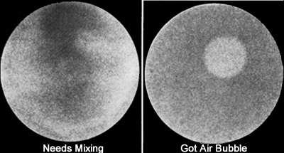
3. Refillable flood is another approach however, there are several issues: (1) larger ones tend to bulge at center, (2) Needs to mixed well, (3) The air bubble needs to burped (look out for the splash), and (4) what about radiation safety?
4. No matter what's in the flood (other than ⁵⁷Co or ^99mTc) uniformity there should never exceed 5% in the planar projection otherwise artifacts will be produced
Intrinsic uniformity
1. Assume that the collimator is not damaged - if you have any question test it - Collimator integrity test
2. Point source should be 5 FOV away from uncollimated detector
3. Amount of activity in the source will vary and you should refer to manufacturer recommendation. According to Elkamhawy et al. deadtime did not degrade uniformity and the acceptable range should be around 0.8 and 3.0 mCi
4. This QC procedure is recommended if the department doesn't purchase a ⁵⁷Co sheet source
5. The only "hassle" is removing the collimator every day to do the procedure
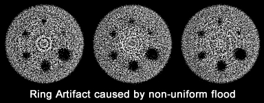
Most common cause of defects in the reconstructed images are due to nonuniformity of the detector. Examples:
1. Correction matrix is the wrong size, correction map is out of date, wrong radioisotope setting, or some form of electronic failure
2. PMT is not functioning
3. Damaged collimator
4. Others?

Jaszczak phantom with reduced imaging time and increased distance

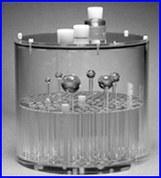
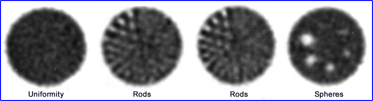
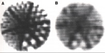
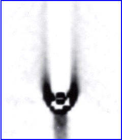
Image acquisition - The above images are of the same phantom, however, "A" defines a SPECT acquisition with optimal imaging parameters, where "B" mimics the clinical setting by reducing imaging time and increasing distance. Test your system with a Jaszczak phantom to find your most optimal imaging parameters
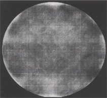
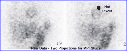
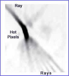
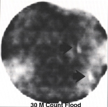
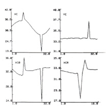
This image shows inadequate differential linearity with the analog to digital computer (ADC). Taking a 30M count image, as in this case, reveal horizontal and vertical lines. Should this occur something wrong with or ADC conversion. How would this affect your SPECT acquisition/reconstruction?

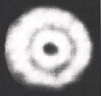
This image can occur when nonuniformity is seen in the imaging system
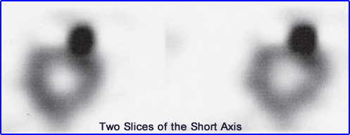
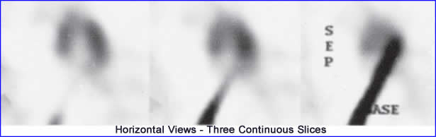
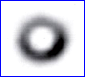
1. The cold circular pattern that appears on the transverse slide of a Jaszczak phantom will happen when (1) improper mixing, (2) air bubble in the refillable flood [less likely], (3) loss of a PMT [most likely]
2. This loss of this uniformity is referred to circular tails or bulls-eye (not related to Van Morrison)
3. What is the other problem that can be identified in the above image? What about the center?

Center of Rotation (COR) and Axis of Rotation (AOR)
1. To correctly reconstruct a 3D image it must be acquired in a 3D format. If the 360 degree acquisition does not collect data in the same dimensional space then artifacts occur. Therefore AOR and COR must be checked and be evaluated routinely
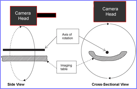
2. AOR is considered the area in which the detector rotates around around a source of activity (line or point or patient)
  1. Detector rotate around the Y-axis - This is what the offset would look like
  2. With a line source placed in the middle of the acquisition the AOR establishes rotational acquisition
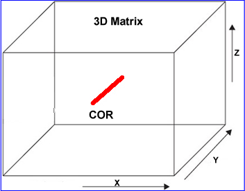
3. The COR is considered the center of the AOR and post acquisition it is displayed within the 3D matrix
  1. COR analysis program will define if there is any misalignment of the AOR
  2. If any correction needs the COR alignment is applied which is referred to as the x-axis offset
4. COR protocol
  1. Distance from the source has no effect on the AOR acquisition
  2. If multiple point sources are required then usually a FOV mask is applied (not required by all systems)
  3. Number of stops is not that important however, 32 projections is recommended
  4. Usually 1 mCi of ^99mTc is considered an adequate amount of activity
  5. Apply 128 matrix and collect between 5 to 20k counts per projection. This usually only takes less than 5 seconds a stop
5. COR analysis
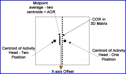
  1. The camera acquires the centroid, the location of the source and displays it. Notice that the two heads (at 180 degrees apart) locates the two centroids in slightly different locations (as seen in the diagram)
  2. The average of the two centroids is the midpoint
  3. The actual COR is shown as a dotted line and the differences between the averaged centroids and the COR. This defines the X-axis offset
  4. Note - we are only talking about 1 set of projections, but in reality COR collects16 data sets (32 stops)
  5. From this analysis the x-axis offset should be <0.5 pixel and requires no correction. However, if 1 or more pixels then a correction is applied
  6. An offsets of greater than 3 pixels requires a service call
6. COR displays
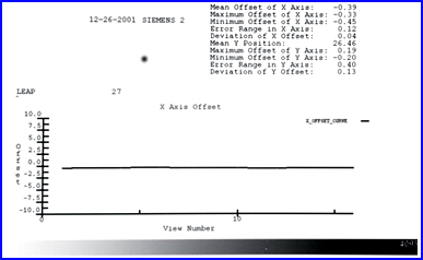
7. This is an acceptable X-axis offset with all data not exceeding 0.5 pixels
  1. Notice some of the data displayed - mean/min/max X-axis offset
  2. What is the true COR offset should be 64.5 +/- 0.5 pixels in a 128 matrix
  3. Y-axis offset can also noted, however, this represents the camera head tilt
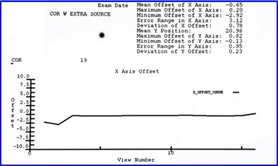
  4. This X-axis offset is an example of an unacceptable COR that has significantly greater than 0.5 pixel variation
8. Sinogram display
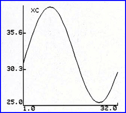
  1. Many COR programs requires the user to place the radioactive source off center so that when the data points are collected a sinogram.
  2. Failure to follow a sinogram path is an indication that the COR has too much variation
  4. Interlocking gears on the rotating gantry causes this abnormal AOR with different COR displays which is what caused the above abnormality
9. Abnormal COR displays
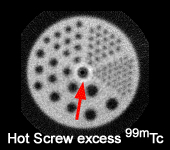
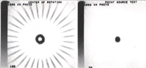
  1. AOR was acquired with the source in the center. The expected results would be a hot spot on the transverse image, however, a donut means that there is problem and in this case it represents a 3-pixel offset
  2. If the same scan is only done in a 180 acquisition then a pitchfork type design is seen. Why does it look this way?
  3. Another example of excessive COR variation shows corrected and uncorrected data
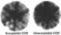
  4. So what happens if a Jaszczak phantom has excessive x-axis offset? Acceptable COR (L) and unacceptable COR (R)
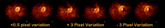
  5. COR display of the short axis in a SPECT cardiac. What is interesting is the intentional off-set of + 3 pixels and - 3 pixels and the type of artifact it generates
10. Misalignment of the COR
  1. With a 0.5 pixel offset occurs image quality is effected resulting in: (1) 30% loss of spatial resolution and (2) 40% loss in contrast
  2. Furthermore, it is recommended that COR analysis be completed on all collimators especially if you are imaging SPECT with medium and high energy collimators. Consider the increased weight on your detector's gantry and how that may effect the AOR
  3. Always keep your detectors parallel to the imaging source because a slight tilt in the AOR will cause a misalignment in the 3D matrix. If this occurs it would be the y-axis that has the offset
  4. Finally, fluctuation of PMTs (or ADC) can amplify a defect while the camera rotates around its axis generating a COR error
  5. Weekly COR checks is recommended as part of your routine QC
Reference scan - Transmission Based Attenuation Correction (TBAC)
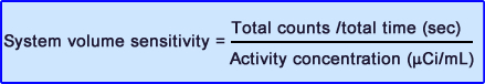
1. Why doe this? Need to assess the attenuation of gamma in air to the surface of the detector. This allows the system to setup the linear attenuation coefficients
2. About the process
  1. Should be completed daily prior to the daily workload
  2. Usually takes no more than 2-minutes to acquire
  3. When acquiring there should be nothing between the reference source and the detector
  4. Acquisition windows acquires data in
    1. Radionuclide being imaged
    2. Transmission source energy
    3. A third window can be set between both imaging peaks to help correct for scatter
  5. If a dual isotope procedure (ex. ²⁰¹Tl and ^99mTc) then then TBAC must be completed with both radionuclide window settings, because there are two energies on-board
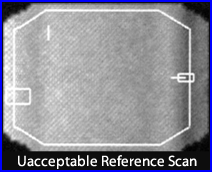
  6. When imaging a patient, once the scan is completed you should evaluate the total counts and uniformity of the reference scan
  7. If a 2-minute reference scan yields <1.8 million counts it needs to be replaced or the shield cover needs to be removed - Why do you think this is necessary?
  8. Uniformity with a TBAC may vary >30% and is considered acceptable since the reference data effects the transmission image at the pixel level
  9. Consider the similarities between TBAC and a uniformity correction map
  10. Examples of reference scans
3. QC comments
  1. Computer program will evaluate total TBAC post patient acquisition to define if there are enough transmission counts
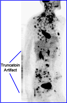
  2. Artifacts can also be generated when the TBAC counts are too low or inappropriate down-scatter correction is applied. If this occurs in real life, the question would be, how does it effect an MPI procedure? Could exaggerated myocardial defect(s)?
  3. Truncation can also generated defects that are not present. How?
    1. What would happen if the patient had barium on-board. How would the TBAC correct for this?
Measuring detector head(s) stability
1. Procedure
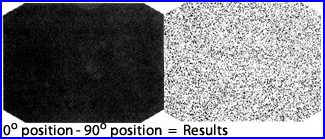
  1. "Tap" your sheet source to the detectors surface
  2. Acquire four images at 90 degrees, around the circle
  3. Set the 0 degree image as a standard and subtract the other images from it, such that you individually evaluate 90^o, 180^o, and 270^o images
  4. Results should display a extremely noisy image with on pattern
  5. This is an partial example of the procedure where the 90 degree image was subtracted into the 0 degree image. Only a noise image remains which gives this camera a passing grade (at least for this angle)
  6. This will identify problems with detector stability that could occur when the camera is acquiring data at different angle
Pixel size calculation
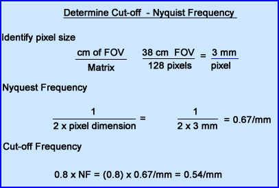
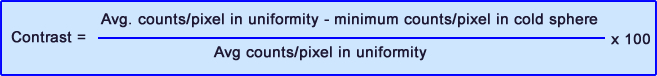
1. This calculation was presented earlier which can be linked here
2. It is important to assure that your X and Y axis are being reconstructed correctly
3. Change in reconstruction filters requires the pixel size data to be correct, within 0.5 pixels
4. Should be evaluated quarterly

Quantitative Application in SPECT

Filter conversion - Filter parameters differ between manufacturers which means that if you want to use the same filter parameters on a different imaging system, then conversion may become necessary. Here is an example of that application
1. The example used is the book is a little misleading - The point that needs to be made is if you know that the NF cut-off is 0.8, then what is its mm value? The is the calculation to make it happen
  1. (1) Determine pixel size - If the FOV of 38 cm and data is acquired at 128 matrix the size = 3mm/pixel
  2. (2) Identify NF = 0.67/mm
  3. (3) Cut-off - If the NF cut-off is set at 0.8, then the mm value becomes 0.54/mm
Spatial resolution and system uniformity
1. Spatial resolution test per AAPM guidelines
  1. Place the line source in the Y-axis of the AOR
  2. Acquire a 360 degree acquisition in a 128 matrix
  3. There should be a 15 cm distance from the source in a circular rotation
  4. Apply a Ramp filter for reconstruction and using the transverse slice determine FMHM and FWTM in the X and Z-axis
  5. Values of both X and Z should be within 1 mm of each other
2. Additional application of spatial resolution
  1. It is also suggested that the line source be acquired in the lateral position with a 10 cm orbit
  2. Also consider applying non-circular acquisition (especially if this is part of your protocol)
  3. Apply this test to every collimator used in SPECT
  4. Reconstruct in all filters normally used in the department
3. Uniformity
  1. While a gallon jug filled with a well mixed solution of ^99mTc this procedure can be used, however, AAPM recommends the use of a Jaszczak phantom
  2. Mixing about 15 mCi of activity set your matrix size to 128 with the same amount of 2D stops
  3. A minimum of 500k counts per 2D is suggested
  4. Reconstruct to a 4 slice thickness using Ramp and Chang and determine integral and differential uniformity
  5. Repeat non-circular and every collimated used in SPECT
  6. Visual evaluation of the ring artifact and calculation of root-mean-square should be done for noise assessment
  7. Integral uniformity should be 10 - 29%
Volume sensitivity
1. Cylindrical phantom with known amount of activity (15 - 20 mCi) with a routine radionuclide used in the department (^99mTc)
2. Count skimming and/or variety is turned off
3. Time is decided and counts are acquired in a pre-set time
4. In the equation apply the acquired values to determine sensitivity
5. When applying the above formula you need to consider
  1. Decay correct total counts at the half way point of acquisition cycle
  2. Axial activity per cm can be determined by dividing the calculated value with the length of the cylinder

Jaszczak Phantom (parts of)
1. This cylinder contains multiple parts of assessment of a SPECT data
2. Composed of Plexiglas it has a 20 cm circumference
3. On the right portion of the diagram it contains a a volume of liquid that is used to determine uniformity
4. Rods extend out with different diameters to test resolution, in the center portion of the phantom
5. The left portion of the cylinder contains cold spheres for further additional resolution evaluation
6. In some phantoms these cold spheres are hollow which allows the user to add an increase amount of activity (over the surrounding media), which contains hot spheres at difference sizes
7. Having hot and cold spheres allows for hot and cold lesion analysis
8. A typical acquisition may include
  1. Circular acquisition with a 64 matrix and 64 stops with a 200k count per injection
  2. Reconstruction is usually done with a Hann or Hamming filter with a NF cutoff of 1.0
  3. Contrast needs to be calculated with the following formula
  4. Range for contrast - 65% largest sphere and 20% small defects
Artifacts generated in SPECT - ray, ring, motion, and truncation
1. Ray artifact
  1. In the FBP reconstruction has a very hot area the reconstruction filters may not be able to compensate for the extreme counts. This can generate abnormality seen as ray(s) in the processed data. Literature also indicates that cold lesions can display a similar effect, but I could not find an example
  2. Backprojection is the culprit and is often seen in just on dimension (or within the 2D plane(s) that it has occurred in). Usually it does not cross over from one transverse slice to the next
  3. In the example below a gated MPI study was collected where the extended R to R wave resulted in a significant drop in counts towards the end of the cardiac cycle. Through imaging normalization the fewer counts became exceeding hot, hence generating a hot spot in the cine and Carrie into the reconstruction process
2. Ring artifact
  1. Any problem that is picked up by the detector via the source or the mechanics of the of the camera can carry through to all 2D images generating a ring artifact
  2. This may relate to collimator damage or non-uniformity in a cylindrical flood
  3. Integral and differential uniformities that get to 5% or more may show a ring (most common reason for this artifact) and is caused by
    1. Non-uniformity that maybe small or centrally located
    2. Poor statistics
  4. COR error or head tilt may be another reason
    
    http://www.spect.com/faq.html
  5. Poor mixing of the radionuclide with the Jaszczak phantom has caused the non-uniformity to appear as rings in the reconstructed transverse slice
  6. This should not be confused with an aliasing artifact
3. Motion artifacts
  1. The effected amount of the artifact depends on: (1) the amount of movement and (2) where it occurs during the acquisition
  2. Movement occurring at the beginning or the end of acquisition tends to reduce this artifact
  3. If the patient or object moves more 2 or more pixels then a clinical artifact will appear on the image
  4. How are the motion artifacts detected?
    1. Evaluate the cine
    2. Generated a summed image
    3. Look at the sino/linogram (best in the vertical direction)
  5. In this example one can see how movement effects the reconstructed images
  6. Here is an example of bladder filling quickly during acquisition that causes an odd shaped bladder. At the same time rays are seen because the reconstruction filter can not compensate for the excessive amount of activity
4. Truncation
  1. Truncation occurs where the reference FOV ends the the emission FOV continues
  2. The extended FOV will not have corrected gamma counts. In PET, excessive counts are seen closer to the skin and these counts can not be corrected
  3. End result is an increase in activity at the surface of the patient
  4. The artifact will more likely occur in: (1) cone/fan-beam collimation (2) bariatric patients
  5. This is example of truncation in a PET scan with a patient that has melanoma. The same principle applies in PET as it does in SPECT. Consider this defect occurring if the patient has cancer located near the surface of the skin
5. Other artifact examples
  1. Collimator integrity
  2. Table/Detector alignment
Acquisition QC
1. Always make sure that patient is positioned correctly (not on an angle)
2. The projection being imaged must be seen on all angles Have you ever acquired a SPECT cardiac where the heart was not seen in all the projected images? What happened to the reconstructed data?
3. Other acquisition abnormalities
  1. Patient’s arm is in the way
  2. Jewelry and belt buckles attenuate the area of interest
  3. Infiltrated dose and a hot spot (secondary hot spot) interferes with the area of interest