A key Points in image reconstruction - each individual image or 2D projection within a SPECT acquisition must be of good quality. Any errors in collecting a single planar projection is magnified in the reconstructed image because each image will contain the error. So if one image has a poorly functioning PMT then ALL 64 images will have the same anomaly. Furthermore when those slices are reconstructed into a 3D matrix the artifact will be manifested and exaggerated.

Hence, any any abnormality or error generated during acquisition will be magnified/intensified in the reconstructed process.

1. First consider the matrix size and its relationship to resolution
   1. Determining the matrix size
   1. For a SPECT procedure the field of view (FOV) matrix size will be either of 64 or 128
   2. Based on sampling theory a pixel size and spatial resolution there are several components to consider
      1. If FWHM is 10 then this value can be divided by 1.75 to give us an idea of what you should be able to resolve down to 5.7 mm - link
      2. In addition, to be able to see a lesion you must cover at least 3 pixels
      3. Furthermore many other factors play into the ability to resolve a small object: distance from object, attenuation, depth of the object, type of collimation, matrix size, and counts
   3. Why don't we acquire a SPECT scan in a 256 matrix? Answer
   4. Factors to consider regarding SPECT and image resolution:
      
      1. The type of orbit acquired greatest effect image resolution: type type is better? Elliptical or circular? What about body contouring?
      2. How does collimation effect image resolution?
      3. Body habitus an issue?
      4. How can zooming help improve image quality?
      5. Energy of the radiopharmaceutical?
   5. Determining the right matrix size for SPECT imaging - your choices are 64 or 128

      FOV	= Widest portion of the imaging field
      Z	= Zoom factor
      N	= Number of pixels (64 or 128)
      D	= Size of pixel

      1. So how do you apply this information? First we need to determine pixel size
      2. Using the above formula let us make several assumptions: camera's FOV = 475 mm , matrix size is 64 x 64 matrix, and no zoom is applied. The result is approximately 7.4 mm per pixel. Applying the rule of 3, if 7.4 is close to 1/3 of the camera's FWHM (assume it's 2.0 cm), then a 64 matrix would be appropriate for this SPECT scan
      3. If you zoom the image by a factor of 1.5 then the pixel size drops to 4.95 mm
      4. If you decide to change the matrix to 128 matrix and not a apply zoom then pixel size is 3.7 mm
   6. Now we need to consider the signal-to-noise ratio and associate this to matrix size
      1. Generally the more noise you have the poorer the imaging quality. SPECT images usually has fewer counts when compared to planar, therefore SPECT images will always contain more noise
      2. Let's crunch some numbers and take a better look at this concept
         1. Assume you collect two sets of images: one at 64 and the other at 128 and both containing the same amount of counts
         2. The 3-D matrix contains 3.84 x 10⁶ counts
         3. How much noise is in these to matrix sizes?
         4. Would it effect image quality?

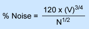
         V	# of voxels in circular FOV
         N	Total counts in 3-D image
         % Noise	Noise generated

         
         
         5. To determine the amount of noise in each matrix the equation above must be applied
         

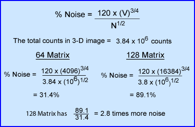
      3. Where V = the amount of pixels in the matrix and N = total counts in the 3D matrix
      4. Crunching the numbers shows us that % noise increases by a factor of 2.8 with the 128 matrix. Hence there is more high frequency noise in the 128 matrix.
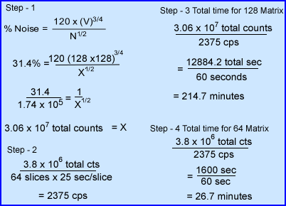
      5. How much longer must you acquire data in a 128 matrix to have the same Signal to Noise Ratio (SNR) found in a 64 matrix? The answer is as follows:
      
      1. Step 1 Counts required for a 128 matrix that would have only 31.4% noise: To determine the amount of counts required in a 128 matrix the same formula would have to used. The differences would be that %noise is known (31.4) and the unknown variable would become N (total counts in 3D matrix)
      2. Step 2 Determine the cps from the acquired 64 matrix: Divide into this value the total acquisition time (slices x 25 seconds/slice) = 2375 cps
      3. Step 3 Acquisition time for 128 matrix: It was determined that 3.47 x 10⁷ counts are needed to have 31.4% noise. Divide into that 2375 cps which give you the total amount of seconds needed to acquire the appropriate count in the 3D matrix. This calculation assumes a constant rate of 2375 cps and does not apply decay. If decay was applied the total acquisition time would increase. The results indicate that a 128 matrix could be acquired in 214.7 minutes
      4. Step 4 - Total time for 64 matrix: Based on the same data it will take only 26.7 minutes to acquire a 3D matrix
      5. Obviously, the time required for the 128 matrix far exceed the any expectation that a patient could tolerate
2. Frequencies and filters
1. Ideally a filter's role is to enhances image quality, without significantly altering the raw components of the input data
1. Incorrect filtering, over or under, can create all sorts of issues, such as: reduces resolution, alter contrast, increase noise (grainy), increase background counts, and/or blurred detailed information
2. Correct filtering ideally enhances the true counts and ignores or removes undesirable low and high frequency data
3. Remember that SPECT images generally have significantly lower counts when compared to planar images
2. In SPECT, image filtering requires the conversion of spatial to the frequency domain which has been discussed in some detail in a prior lecture. Click here to review
3. Perhaps, at this point our concern should focus on how to optimize the computer ability to convert frequency domain which is done by defining and working with the Nyquist Frequency (NF)
1. Why is the NF so important? Think of NF as if it we're trying to record something. To do so we must record a representation of all possible sound. You could say that we are attempting to record the entire band width of sound. In essence, Nyquist represents an entire spectrum in the frequency domain. Therefore, in a SPECT study we must consider this concept by setting the correct NF so that we can visualize the entire spectrum of spatial data in the frequency domain
2. Therefore, NF takes into account ALL frequencies which we can break down to the follow components:
   1. Low frequency is comprised of background and large objects
   2. Middle frequencies are variation of smaller objects. As the object continue to get smaller the frequency continues to get higher
   3. High frequencies - small to very small objects plus noise. It may be difficult to differentiate between very small objects and noise because, especially when the they system reaches its FWHM
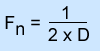
3. An optimal sampling for NF is to place two pixels into one complete cycle by applying the following formula

Fn	Nyquist Frequency
D	Size of Pixel

4. The formula defines NF with the symbols F_n and relates it to pixel size and applies the number 2 since it wants to fit an entire cycle into 2 pixels. The actually value of NF will be displayed in cycles per mm. Let us apply some numbers to see how this works. From our previous work (determining the appropriate pixel size for SPECT) let us revisit the 475 mm FOV camera
   1. If we apply the 7.4 mm pixel in the 64 x 64 matrix to the above formula the NF becomes 0.06868 cycles per mm^-1
   2. So what does this mean? This means that in order capture the best spatial frequency the NF must be set at 0.068 cycles/mm^-1. To go beyond this point means we would be able to see an even smaller object, but in reality to go beyond that point means that we are seeing nothing but noise
   3. Note that the pixel value, D, must be twice per cycle it is for that reason that the value is multiplied by 2
   4. If a 128 matrix is used with a pixel size of 3.7 mm the NF becomes 0.16 cycles/mm^-1
   5. Applying NF to image filtering and FBP - reconstructing SPECT data you must work within its Nyquist and apply the entire frequency!
   6. Warning - NF will very if the FOV is magnified - See pixel size
5. More comments on NF
   1. Manufacturers define NF in several different ways, two that come to mind are: cycles/mm and cycles/pixel
   2. The above calculations was done in cycles/mm, however, it maybe more appropriate to consider NF in cycles/pixel
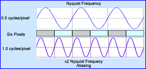
   3. Why? This is because the maximum NF will always be 0.5 cycles/pixel. The reason for this is that it takes two pixels to capture the entire cycle
   4. Too many waves in a pixel set causes aliasing that is a result of mis-matched frequencies. If the frequency is >0.5 then high frequencies spill into low frequency data
   

6. Therefore, whenever we filter an image in SPECT it is necessary to always work with the NF framework. Failure to not include all of it would result in not capturing all information that is available for processing
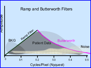
   1. The images above show the correct NF at 0.5 cycles/pixel, where 2 pixels capture the entire cycle. An example of over sampling is also noted when the NF is set to 1.0 cycles/pixel. What happens if over sampling occurs? (I would assume that what you might be trying to capture is even smaller objects?) Well it doesn't work! Look below
   
   
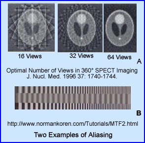
   A - Shows a set of images taken with different amount of acquired SPECT slices: 16, 32, and 64. Notice the "squares" seen in the data. This Moire type defect is seen more clearly in the background of the transverse slice, but also within the brain phantom. This is known as aliasing. The generation of this artifact is not specifically from over sampling, however, the end result is the same, aliasing

   B - Shows a set bars with variation in size. Aliasing, in the center of the strip, specifically were the bars just don't line up. This occurred because the NF was set at 1.0 cycles/pixel

3. What's in the frequency? We've discuss it prior to this lecture, but now for the details

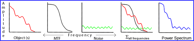
1. The frequency of an object or objects has several parameters the need to be understood for the learner to comprehend what he/she is truly looking at when evaluating data that has been converted to the frequency domain. Hence the display of different frequencies, all of which where acquired from the same data source.
   1. Object(s) - have specific frequencies that are of different sizes and contain different levels of radiopharmaceutical uptake. These variations within the downward slope denotes statistical fluctuation of the acquired objects. You should be able to define where the large/mid size/small objects are located within the graph. In addition, based on this graph you should be able to define where the smaller objects can no longer be visualized
   2. MTF - Displays the camera's maximum ability to resolve an object. Furthermore, you should appreciate that resolution can never be at its maximum when acquiring SPECT data from a patient. Therefore, hypothetically you will never be able to maximize the system's resolution. Why?
   3. Noise - The amount of noise depends on the amount of counts collected in the acquired data and which matrix size the data has been acquired in. At the point where noise and the objects' resolution collide is the point where spatial resolution is lost. Why is the a true statement?
   4. Power Spectrum - is the summation of all frequencies acquired from the spatial domain. It is what you would actually see if you pulled up the acquired data on the computer
2. Remember the variables that effect imagine resolution and apply that information to the data seen above: collimation, patient to detector distance, type of acquisition orbit, Compton scatter, body habitus, and the type of reconstruction selected to evaluate your 3D data
3. The low/high frequencies issues
   1. The smaller the object
   2. The fewer the counts the greater the noise and grainy. However, the more the counts the less noise there is. Noise and small objects can become lost in the data which can potential cause us to miss disease
   3. Low end frequency issues might normally be considered background and scatter issues, however, Poisson statistics "blurs" or "smooths" critical data in the low frequency domain as noted in FBP reconstruction. Therefore larger objects with poor radiopharmaceutical objects may be removed and cause a false reading

   

4. How does an increase in your count density effect image resolution?
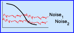
   1. The frequency curves that are displayed above include: MTF of the gamma camera (black) with two separate acquisitions seen in red. Both sets of data were acquired over the same object, however, Noise₁ has has a lower count density
   2. Both sets of data show similar low frequency fluctuation
   3. However, since Noise₁ has a lower count density resolution is lost sooner because noise interferes into lower frequencies causing a loss of resolution
   4. Noise₂ has a higher count density so it allows the physician to evaluate disease and objects that are smaller in size
   5. Therefore
      1. The more counts you acquire the better your resolution via less statistical variation the
      2. The goal, if attainable would be to utilize the camera's MTF to its fullest potential
      3. However, as noted earlier to apply a 128 matrix (better resolution) and have the same amount of noise in a 64 matrix the acquisition time would take hours instead of minutes
      4. Finally, the longer your acquisition time, the greater the probability that the patient is going to move
4. Filtering process in SPECT
1. Pre-filter the raw data
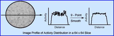
   1. Many places actually pre-filter the raw data, which means that each 2-D images within the 180 or 360 degree rotation are filtered prior to reconstruction. Why is this recommended?

   

   2. The rational for this is simple - If you are dealing with low count images then you're going to have a lot of high noise. By completing a 9-point smooth on each 2-D slices you removing excessive fluctuation in the high frequency range. An image profile, before and after smoothing is noted
2. Overview on the types of filtering used in image reconstruction
1. When filtering the backprojection during image reconstruction there are several basic aspects that filters must accomplish that will eliminate unwanted data
   1. Removal of BKG
   2. Removal of noise
2. The three basic types of filter that accomplish these two task
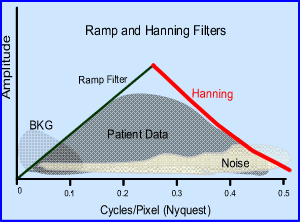
   1. Low pass filters suppress high frequencies and amplify low frequencies. Examples would include: Hamm and Hanning filters
   2. High pass filters do the opposite, that is it suppresses low frequencies and amplifies high frequencies. An example of this type of filter would be Ramp
   3. Band pass filter suppress low and high frequencies and amplify mid-range frequencies
   4. It should also be noted that whatever is adjusted during image reconstruction we have no specific control! When you cut off noise and/or background you may eliminate to much or not enough of either or both. At the same time when you eliminate too much you may also be removing true counts.
3. Restoration filters attempt to restore data and improve the quality of the image. Two examples would include Wiener and Metz
4. Partial volume (or Surface) rendering allows the user to create a 3-D surface image of an organ that has been acquired through SPECT. Generally this may not be considered very useful since it is unable to look inside the structure. However, analyzes of external (surface) anatomy may be beneficial. As an example might be a the brain where "hole" on the surface could be do to infarct or tumor
5. Post-filtering (after reconstruction) may also be applied, especially if the end results from reconstruction contain a lot of noise. Iterative reconstruction tends to have more noise post reconstruction and an additional smoothing filter may be recommended
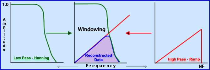
3. Filter reconstruction with high pass filter
1. Ramp filter is recommended - Two issues to consider



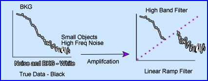
1. The main role of the linear ramp filter is to amplify the high frequency to better resolve the data. In addition, lower frequencies are suppressed. Notice how the filter "cuts" right through the middle of the curve. Comment - if the entire frequency was amplified then true counts, BKG, and noise would all be amplified. This would serve no purpose
2. Not only is BKG removed but so is image blurriness so. Hence, the ramp filter cuts off the low frequency background, which removes unwanted data. This is good! Removing low frequency also removes image blurriness and the star defect
3. What remains in are true counts + high frequency noise
4. What what do we do with the noise?
2. Add a low pass filter to the process
   1. By applying a Hanning filter (as an example) you are now able to suppress high frequencies
   2. The goal is to suppress both unwanted low and high frequencies and the term "windowing " may be used. In the end the hope is to have only true counts that can then be applied to the image reconstruction process. However, the reality is that sometimes our approach is a trial and error with minor frequency adjustments, before you actually get the desired results
   
   3. Here is example of applying low and high frequency filters. In this application the Ramp removes low end frequencies and when you add the Hanning it "roll off" the ramp resulting in the removal of unwanted high 0Sfrequencies
3. What about band pass filters?
1. Another approach to this window technique to to use one filter that removes high and low frequencies. Again the goal is to have only true counts in the reconstructed data
2. Butterworth filter has this capability and is perhaps one of the most popular filters used in the nuclear medicine community
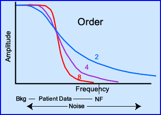
3. It also has specific characteristics that require further discussion: critical frequencies and order (power)
4. Butterworth filter
   
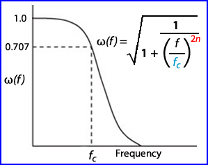
   1. The variables the influence the Butterworth filter are critical frequency (fc), order (n), and power (2n)
   
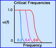
   2. Critical frequency adjustment is completed by manipulating the Butterworth formula (fc). By changing it from 0.2 to 0.6 you can extends the x-axis of the graph outward, increasing the level of at the MTF to identify objects, but it maintains contrast (the slope does not vary significantly. Comment on an object's visibility - large objects to small
5. Filters and there orders

1. Some filters, such as the Butterworth (n in the formula), allow you to adjust its order. Essentially this change the slope on the filter. In the case above, when you increase the order number, increase the negative component of the slope, adjusting contrast
2. This manipulation allows the user to remove or add difference frequencies to the reconstructed image
3. Note that an order of 8 increases the amount of lower frequencies, but doesn't accept as many frequencies at the higher end. While decreasing the order number reduces the amount of lower frequencies, but accepts more frequencies
4. To accept more lower frequencies and reduce high end creates a more blurry/smooth image. Doing the opposite causes a grainy/noise image
5. Yet a second element to all this is considering image contrast. The steeper the slope, the shorter the transition zone, of the curve the greater the response is to contrast, while a less negative slope has has a more gradual change in imagine contrast
6. Some literature refers to this as the "power" represented by 2n in the formula
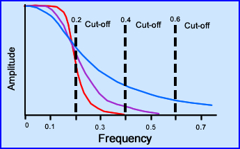
6. Cut-offs - Is an additional application used in filter reconstruction

1. Another component to all this adjustment is to apply a cut-off frequency. In the above example the same Butterworth filter is applied with the orders of 2, 4, and 8
2. At this point your goal should be to apply a cut-off that removes unwanted frequencies that only contain noise
3. Note the affects of the different cut-offs above. If you look at 0.4 you can see how it eliminates all the higher frequencies but may also limit the amount of true counts. Of the three cut-offs represented 0.4 would be the most acceptable. Why?
4. By adjusting the cut-off we can effective eliminates high frequency noise leaving BKG and true count data. This improves image quality via the elimination of statistical noise at the high end reducing the amount of graininess in the image
5. Finally, it is usually recommended that you set the cut-off to 0.5 cycles/pixel. This was mentioned mentioned earlier during the lecture. Why do we want to set the cut-off at 0.5?
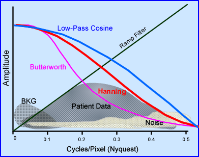
7. Combining Ramp filters
1. The key is to be able to remove as much of the unwanted frequencies as possible. Hence, the application of both low and high filters is required



2. First apply the Ramp filter to remove low frequencies
3. The window it with any one of the low frequency filters. Which one gives you the best results when windowing the frequencies?
4. Given the previous graphs I have selected two different sets of windows for review. Which of these two combinations is best suits for the reconstructed criteria?
4. Let's spend a little more time discussing other types of filters
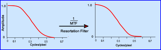
   1. How do restoration filters work?
      1. The concept is to improve resolution on a low count by restoring counts in an image. Hence, images with low count density may benefit with this type of application
      2. There are two types that we will discuss: Wiener and Metz
      3. Application of concept
         1. Metz filter works similar to ramp in that it amplifies frequencies, but an inverse MTF causing the amplification of low and mid-frequencies instead of the higher frequencies
         
         2. The above image shows what happens with the filter that takes the MTF and inverts it. Once this is accomplished the mid and low frequencies are amplified
      4. Wiener as another type of restoration and it works on a different principle
         1. It's goal is to filter out noise and it is noise that corrupts the patients counts within data that contains the true counts
         2. By applying an SNR concept this filter assumes that signal and noise are linear and its probable distribution can be identified
         3. Using the statistical concept of "minimum mean-squared error" noise is eliminated from the signal
         4. Another way to think of this is to assume that the frequency data has multiple convolutions based on the spatial frequencies in an image
         5. If convoluting noise is identified, then just subtract via deconvoluting the noise. Or apply a reverse wave/cycle of noise will result in data containing true counts
         6. Use this hyper link to find out more about Wiener filters
   2. Creating a three-dimensional image
      1. Surface rending filters allow the user to look at a three dimensional surface. Application may include heart or brain, where evaluation of the surface might lead to the detection of lesions that incorporate the surface of the organ
      2. To accomplish process the filter looks for a certain count threshold within the 3-D matrix. As the activity exceeds BKG then an "edge" is detected defining a solid surface
         
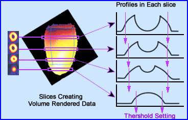
         1. As the example above shows the threshold set in such a manner that a count profile can identify the edge of the LV. Once all 2-D slices have been evaluated a boundary tracking algorithm lines the slices into a volumetric image
         2. Also referred to as edge detection the volume of the left ventricle is drawn
      3. Volume rendering is then used to display the images either as static 2-D or 3-D rotation where the viewer can use the mouse to rotate the LV to any angle, see below
      4. The most popular type is known as Maximum Intensity Projection (MIP)
         1. The difference, here is that instead of finding "hottest" voxel in a count profile or line, MPI looks for the hottest voxel in a ray, where the one with the most count density because the edge of the organ
         2. These rays with the hottest voxels are then connect and form a 3-D image
         
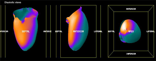
         3. This display shows the LV of the heart which can be manipulation to view any angle with the touch of the mouse. However, it cannot be displayed in this web based program (sorry)

         

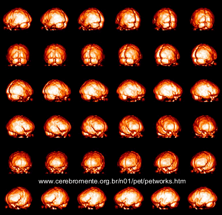
         4. Another example of surface rendering shows a brain scan. Ideally this display can be shown as a cine or as a single image where the mouse arrow can be drag to display the brain at any angle
         5. Most programs allow you to rotate the single picture to any angle the user wishes to look at
            1. Advantage of this approach is to identify any abnormalities on the surface of the organ
            2. Disadvantage is simple - you cannot see beyond the surface
5. Display of the reconstructed data
   
   1. Images displayed in the most typical format (cardiac is the exception) allows the viewer to display the planes of body: transfer, coronal, sagittal
      1. The above image is color coded to help you appreciate 3 planes of the body
      2. Transfers is green, coronal is blue, and sagittal is red
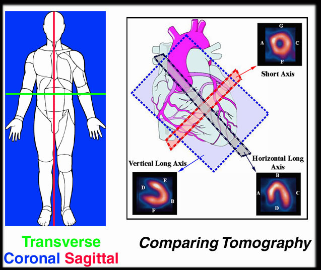
   2. In the heart requires a modification to the "right angle" approach just mentions
      1. the oblique orientation of the heart means that your typical transverse, coronal, and sagittal slice just cannot apply (wrong orientation)
      2. To evaluate the heart in a different orthogonal plane the 3-D matrix is rotated and reorientated to the appropriate angle
      3. Tri-linear interpolation is applied which smooths the voxel in all dimensions and then the voxels count densities are identified and the images are then reconstructed
      4. This smoothing operation does cause some minor lost to resolution
      5. In the heart these changes in orientation create three different angles: vertical long, horizontal long, and short axis
   3. Dynamic triangulation
      
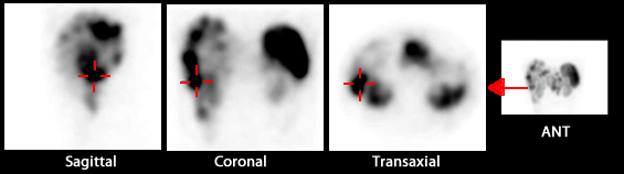
      1. The arrow pointing out from the ANT image is the lesion in question.
      2. Finding the disease in any one plane shows the corresponding other two planes within the same 3D space confirming the lesion
   4. Cine mode can be seen in SPECT in either rotating the raw data or cardiac wall motion

Return to the beginning of the document
Return to the Table Of Contents
3/ 23

Chapter 10, The Essential Physics of Medical Imaging,Bushberg Radiation Detection and Measurement, Knoll, 2nd ed. http://engineering.dartmouth.edu/courses/engs167/11%20Image%20Analysis.pdf