Basic CT - Making the PET Connection

1. This lecture is a review and discussion on the general principles of a CT scanner. There is no better way to understand how a CT scanner works than to look at the original CT scanner. Textbooks refer to this as the first generation CT, the original scanner



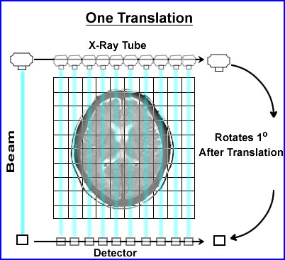
1. When CT was first developed its collimated x-ray beam was 3mm thick and 13mm wide. On the opposing side was a single detector which recorded the attenuated beam
2. The beam would swipe across the patient, in a linear fashion, collecting the attenuated data. Then data collected within the slice was referred to as a single translation
3. Once the translation was acquired the x-ray tube and detector would move 1^o and repeat the linear transmission collecting its second translation
4. In the original scanner a single translation contained 160 rays (or x-ray beams) of data. In today's technology there are at least a 1000 rays within a single translation
5. This first generation CT acquired 180 views (completing 1/2 a circle), stepping around the patient collecting data in a semicircle. This information would contained 360 degrees of data
6. This process was considered slow (compared to today's technology) and would take about 6 seconds to complete. That is 1 - 180 set of translations
1. Acquisition and reconstruction
1. Remember the concept of pixels and voxels from our SPECT lectures - consider CT having a similar application
2. The similarity being our ability to image 3 dimensional space, however, instead of physiological analysis, anatomical data is collected
3. Collecting counting, or x-rays from CT, evaluates the amount of attenuation that occurs with each emitted x-ray. The type of attenuation being evaluated is referred to as linear attenuation coefficients (μ). So instead of counts we are counting x-rays
4. The variation in μ occurs when tissue densities vary within the 3D space
5. As a general rule, a CT matrix size is 512 x 512 or 1024 x 1024 with a thickness of 0.5mm². Adding the third dimensional space turns the pixel data to a voxel. The size of voxel is usually around 1mm or smaller
6. Once the data is acquired, in the matrix, it is usually referred to as a reconstruction matrix
7. Image matrix is then interpolated from the reconstruction matrix, where display adjustments are applied, such as zoom and/or filters
8. Generating the reconstruction matrix



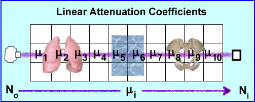
1. N_o is the production of the x-ray that travels through 3D space (example above shows 10 voxels)
2. Depending of the amount of density encounters (air, liquid, and/or bone) there will be a variation in the ray's attenuation. These values of attenuation is referred to as u_i where the beam may encounter different degrees of attenuation within a certain volume of voxels. The end point of the attenuated ray is then referred to N_i were the detector records the amount of attenuation. End results - linear attenuation coefficient
   , μ, that occurs from that specific x-ray
3. Given the chart above different attenuation coefficients are displayed. These attenuations are based on a 100 kVp beam. It should be further appreciated that a typical CT tube generates a poly-energenic beam within the 100kVp . Its energy variation (kVp) is approximately 1%. Furthermore, a CT x-ray beam can be adjusted to a low of 70 kVp and a high of 140 kVp
4. The attenuated sum (X_n) occurs after the initial ray N_o passes through a set of voxels which in turn becomes N_i and can written as X_i = ^_ ln(N_i/N_o). In addition, X_i represents a specific number of voxels within the ray and because it is 3D it becomes w_i, where w stands for width (amount of voxel).
5. Hence the attenuated ray is the sum of only 1 ray traveling across a set of voxels in 3D space. There are 160 ray that makes up 1 translation and 180 translations makes up one axial acquisition. One might say, "that's a lot of data"
6. While a CT scanner calibrates its linear attenuation coefficients by initially "cutting air" via a QC procedure, yet the "magical" number/value for CT is considered water. Why the value of water so important?



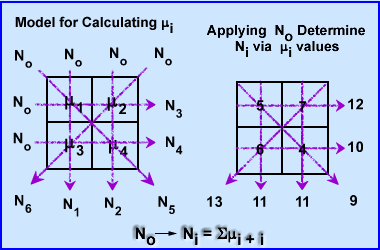
9. (You are not responsible for this section, but I found it interesting on how CT actually determines the μ value in a voxel) How does a CT scanner determine the μ values in 3 dimensional space? To simplify the process let us look at a 2 x 2 matrix using an iterative algorithmic approach, Algebraic Reconstruction Technique (ART)
   1. The attenuation in these 4 pixels are hypothetically unknown, however, when you apply an x-ray beam to them, N_o, at six different angles, 6 N_i, the values are detected (N_1-6). This is demonstrated above

   

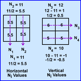
   2. To find the μ values we first sum both rays at 0 degrees. N_1-2 rays have the same summation 11. Since 11 is the sum of 2 pixels within each ray it is divided by 2 making the attenuation 5.5 for N₁ and N₂. This : value is placed into all four pixel.
   3. To find the at 90 degrees ray N₃ summation is 12 which is then subtracted by sum of N₁ (11) and divided by its 2 pixels (N₃ - N₁/2). The value is +0.5 which tells us to add 0.5 to each pixel in the N₃ ray. The same process is applied the other ray N₄, with the final value being -0.5 (N₄ - N₂/2). We now subtract 0.5 in the 2 pixels that compose the N₄ ray

   

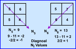
   4. At 135 degrees N₅ ray sum 9 and when subtracted from the N₁ it becomes -2. Because there are 2 pixels in the ray this value is divided by 2 has a difference of -1.0. We then subtract 1 from each pixel within that ray (N₅ - N₁/2)
   5. At 235 degrees N₆ has a final value of 13, subtracted by 11 gives a value of 2. Divided by the 2 pixels requires to addition of 1.0 to each pixel. (N₆ - N₂/2)
   6. The end result shows us that the ART method can correctly determine attenuation values
   7. Now imagine if you will, these calculations being applied to a 512 x 512 matrix in 3 dimensional space
10. (Back to what you should know) Backprojection (Remember FBP?)

    

    1. Once the attenuated values are determined these coefficients must be backprojected, as in a SPECT image, however, instead of CT counts the attenuated x-rays values are being applied
    2. These attenuated values are displayed evenly across each backprojected ray, 180 degrees around the patient
    3. Looking at the above image 2 attenuated objects have been placed in the volume. The image to the left shows x-rays being projected and detected. The image on the right are the backprojected rays
    4. Backprojection causes the image to be blurry (just like SPECT) and therefore image filtering must be done.
    5. Graininess in CT is referred to as quantum mottle which occurs when there are too few x-rays/voxel. In nuclear medicine we can relate this concept to low count imaging
    
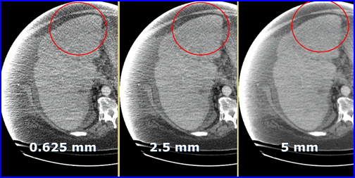
    6. Here is an example of quantum mottle in a patient with excess attenuation. The problem is solved by increasing the thickness of the slice. Why does the increase of slice thickness improve image quality?
    7. The fewer the rays the greater the noise
    8. Spatial resolution is improved by image filtering (just like FBP in SPECT) because it reduce noise and improves contrast.
    9. CT is able to see a lot of detail, however, if different surrounding structures are similar in their attenuation value, which could include background and noise, detail becomes difficult to resolve. This is because of there is little difference in the surrounding media, little variation in μ. To solve this problem CT uses a concept referred to as windowing



11. Windowing - A gray scale adjustment
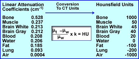
    1. Linear attenuation coefficients can be related to another term known as House-field Units (HU). These units vary from -1000 to 1000 (very dense one can go beyond 1000, ex. metal), with water having the value of 0. Once μ is determined HU values can be calculated from the above formula. This is applied to a gray scale on the final image. Several : are noted above with their respective HU values. The formula above can also be used to convert from : to HU
    2. Windowing has a effect on the gray scale
    3. Consider that most areas being scanned will be have a range of 2000 HU, but there are only 256 shades of gray. If you wanted to apply the entire 2000 HU to 256 shades of gray this would mean that every gray would cage after every ~8 HUs. Hence, slight changes in density say via the initial invasion of disease might be missed
    4. Therefore, windowing is applied, in which HU only looks at a small variation within the attenuation range. This allows shades of gray to be more affective in finding small variations in tissue density (this also improves contrast)
    5. The following is an example for adjusting the window level (WL) and window width (WW) . Where the WL is considered the midpoint (or peak if we were talking nuclear) and WW is the length of the opening (or percent window if we were talking nuclear)

    

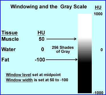
    6. The above is an example of where WL would be set at -25 and the WW is 150. Divide 150 by 2 = ±75 placing the window width at 50 HU to -100 HU
    7. When the operator selects a specific tissue type it sets a WL at the midpoint of the HU and gray scale. Examples¹ of suggested values
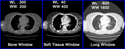
       1. Examples of different settings from Radiopaedia website - click it

    
    http://rsbweb.nih.gov/ij/plugins/ct-window-level/index.html

    8. Selecting the right window becomes critical in finding disease in different structures of the body. Consider brain vs. bone and note the degree of density between both organs. The two windows that apply are soft tissue and bone respectively
    9. In the above example for bone window the WL is set at 300 HU and the WL is set at +/- 150 HU @ 200 HU
    10. Important to note - selecting the window width defines the amount of contrast and is referred to the "gray-scale rendition of specified tissue."
2. Other technical aspects of CT development
1. In the literature CT development is usually referred to as 2^nd, 3^rd, 4^th, generation, however, for our limited review, I will look at how CT scanning improved over time. The key to most of CT development is to reduced scanning time that allows for the evaluation of a more dynamic model
   1. Single narrow beam with a detector evolved to three beams/three detectors on the same gantry. However, anything more tubes/detectors, beyond three, created too much gantry motion
   2. Thin beam became fan beam which encompassed the entire patient's width. Thus further reducing the scanning time by increasing the imaging area so that the entire diameter of the patient was covered in one translation. In addition, fixed detectors were set at 360 degrees around the scanner, so that only the x-ray tube moved

   

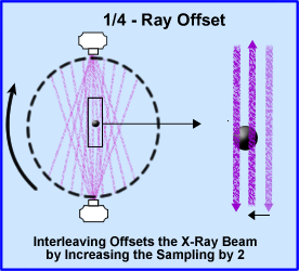
   3. 1/4 - ray offset takes the concept of doubling your sampling size by increasing the amount of x-rays going through the object by two. In addition the scanner rotated 360 degrees around the patient. The diagram shows beams sampling around the object. The second beam samples the object at 1/2 the distance from the opposite direction, hence interleaving the object and improving image resolution
   4. Reducing the time an x-ray goes through the patient by increasing speed and energy of the x-ray tube allowed CT analysis of the myocardium

   

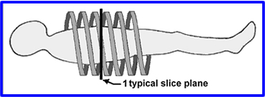
   5. Slip Ring and Helical CT - In prior technology cables limit the rotation of the gantry. The scanner could spin in one direction, but then it would have to D-spin so it can spin again. By using a drum, grooves with metal brushes to "connect" the electricity, cables were no longer required allowing a CT scanner to spin in either director without having to unravel itself. Additionally, the scanner would spin in a spiral pattern, never overlap.
      1. Helical pitch is used to define the table movement per rotation divided by the slices thickness
      2. Example: If a slice thickness is 5mm and the table moves 5mm per rotation then this equal to a pitch of 1.0
      3. A pitch of 1.0 means no over sampling, however,
      4. If you go beyond a pitch on1.0 then areas become under sampled and estimations of the missing tissue must render an estimated μ values
      5. Another concern - if the table moves too fast then there may be a motion artifact
2. Technical points to remember

1. CT uses a beam that generated around 100 to 140kVp = 100 to 140keV
2. Beam hardening occurs when an x-ray beam penetrate deeply into an object. The more density translates to greater Compton and Photoelectric effect. This causes the center of this object to be darker because fewer x-rays are recorded. In SPECT we call this cupping
3. Septas are used in CT and are placed between detectors. This reduces scatter of the attenuated beam and improves contrast
4. Quantum mottle is a low count image in nuclear

The Beginning of the Document
Next Lecture - PET/CT Imaging Artifacts
Return to the Table of Content

2/24

Most of this this lecture came from the following articlePrinciples of CT and CT Technology by Lee W. Goldman, Journal of Nuclear Medicine Technology Volume 35, Number 3, 2007 115-128

1 - Value of bone window images in routine brain CT: Examinations beyond trauma by BA Georgy, et. al .