
Visualizing Data
Creating a Graph
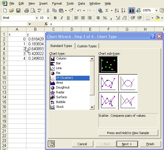
For our purposes a graph requires two columns of data, the input and the corresponding output from a function. Examples of how to set this up can be found on Page 2. Graphs can be relatively simple or fairly elaborate (with labels for the data and axes, a title, a legend, and various gridlines and tickmarks), but we will stick with the basics. All we need to do is select the x and y ranges (together or separately, holding down the CTRL key) then click on the Chart Wizard (the button with an icon representing a bar chart).
 Obviously
there are a great number of different types of charts possible, but we
are primarily interested in the XY (Scatter) option. Anything else will
graph the x and y columns separately rather than x versus y that we want.
You can then choose whether you want to connect the points and click on
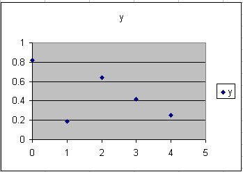
Finish. The result is not necessarily beautiful, but quite functional
(pun intended).
Obviously
there are a great number of different types of charts possible, but we
are primarily interested in the XY (Scatter) option. Anything else will
graph the x and y columns separately rather than x versus y that we want.
You can then choose whether you want to connect the points and click on
Finish. The result is not necessarily beautiful, but quite functional
(pun intended).
You will notice that it automatically generated a title
and a legend, using whatever label you typed at the top of the y column.
The legend is useful if you have more than one y column to display (they
will show up with different colors and point styles), otherwise you can
just click on it and hit the DELETE key to get rid of it.
Manipulating Graphed Data
Having created a chart, once you click on it to select it, several things happen. First the chart sprouts "resize" handles that you can drag to modify the dimensions of the chart. Second, a Chart menu appears on the menubar. Under this menu are a number of formatting options, with which you can always go in and add stuff that you skipped in the initial Chart Wizard by clicking Finish right away. You can also get to these options by right-clicking on the chart. Finally, you will see colored borders appear around the data that the chart uses.
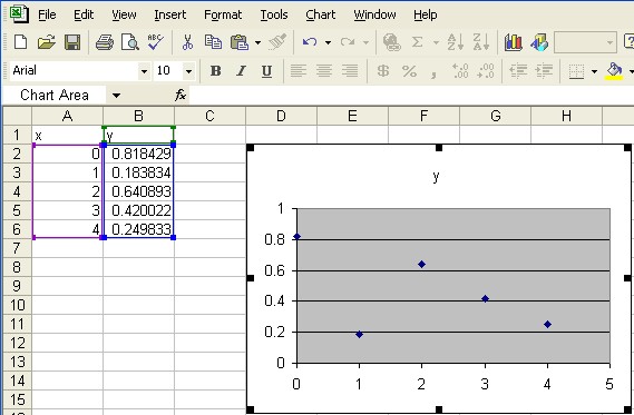
If the data in these highlighted ranges changes, then the graph will change (useful for experimenting). But even more useful, if you should decide to add a few more x and y values in your columns, you can stretch the colored borders to include the new points by dragging down on one of the bottom handles. If you want to restrict your graph to the same number of points but use different ranges you can just click on the edge of the border and drag it to highlight a different set of points. If you want to add a whole new column of y values next to the original one you can stretch the highlighted border sideways by dragging the right corner to include the new column of data.
Graphs with Multiple Functions
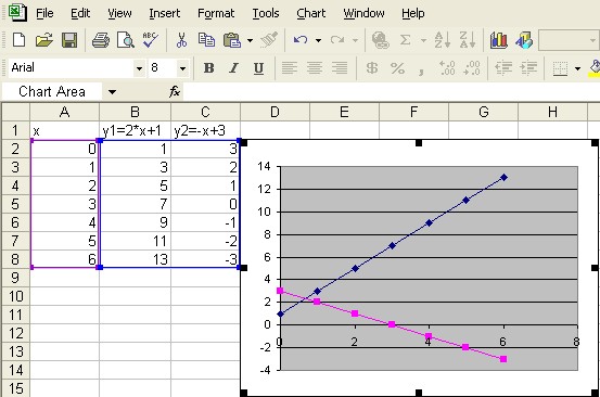
As indicated right above, if you want to compare two functions on the same graph (either to see how they are different or to see where they intersect), you would generate three columns of data. One column would be the x as before, and then there would by two y columns, one for each function. You can generate these y columns with different calculations.
 To
actually create this chart the only thing you do differently is to select/highlight
all three columns of data before you click on the Chart Wizard. It also
helps to choose to join the points. Even though Excel automatically uses
different point styles for different sets of data, all those points can
get confusing without lines connecting them.
To
actually create this chart the only thing you do differently is to select/highlight
all three columns of data before you click on the Chart Wizard. It also
helps to choose to join the points. Even though Excel automatically uses
different point styles for different sets of data, all those points can
get confusing without lines connecting them.
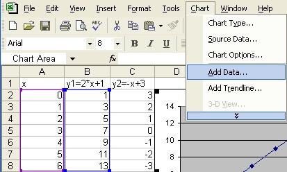
If you already have a graph with one set of data and you
want to add another you can either do it using the handles on the blue
border highlighting the one column of y values and drag it to include
the other column, or you can use the Add Data... option on the Chart menu.
This will explicitly ask you for the range of addresses (e.g., C2:C8 here)
where it can find the new set of y values. You can either type in the
addresses manually or go out and select them with the cursor.
Finding Equations from Graphs
 Sometimes
you start with the equation for a function and you want to see what it
looks like by calculating points and graphing them. At other times you
merely have a bunch of points and you don't know either what they look
like or what equation might represent them. This is often the case when
dealing with empirical observations. It turns out that Excel can be used
as a tool to derive the appropriate equation for a given set of data using
something called a "trendline." To calculate and display the
trendline you proceed as before. Type in the x and y columns, select them
and click on the Chart Wizard to create the graph. Once you have a graph
you can select it and look on the Chart menu (see above) for the Add Trendline...
option.
Sometimes
you start with the equation for a function and you want to see what it
looks like by calculating points and graphing them. At other times you
merely have a bunch of points and you don't know either what they look
like or what equation might represent them. This is often the case when
dealing with empirical observations. It turns out that Excel can be used
as a tool to derive the appropriate equation for a given set of data using
something called a "trendline." To calculate and display the
trendline you proceed as before. Type in the x and y columns, select them
and click on the Chart Wizard to create the graph. Once you have a graph
you can select it and look on the Chart menu (see above) for the Add Trendline...
option.
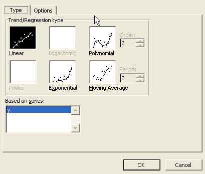
You will be presented with several different possible types of functions. Some of them are already ruled out because of the way they behave when x=0. However, you need to have some idea what your function does or should look like. Most of the time we are interested in a "linear regression," the first option, which is the straight line that comes closest to all the points.
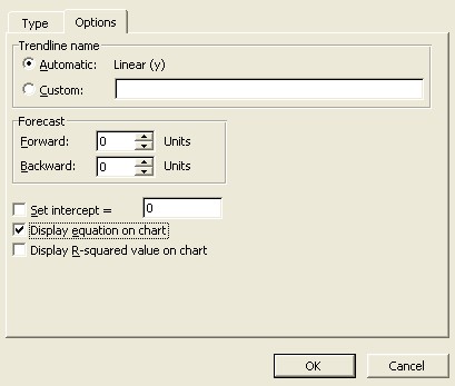 If
you hit OK right now, Excel will draw the line on the graph, but not tell
you anything about it. To find the actual formula/equation and display
it on the chart as well, go to the Options tab and place a checkmark next
to "Display equation on chart". Then you can click on OK.
If
you hit OK right now, Excel will draw the line on the graph, but not tell
you anything about it. To find the actual formula/equation and display
it on the chart as well, go to the Options tab and place a checkmark next
to "Display equation on chart". Then you can click on OK.
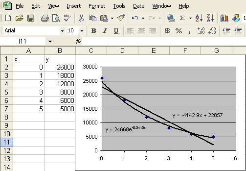
It is possible to put more than one trendline on the same
chart, just repeat the process for whatever kinds of functions you think
might work. When you are done you can look at them and decide which one
does a better job describing the data. In the example below a linear function
and an exponential function were attempted and it is fairly clear that
the curved exponential function matches the levelling off effect in the
data better. You can get a quantitative measurement of how good your function
is by checking the "Display R-squarted value on chart" under
the Options tab. The closer to 1.0 this value is, the better your function
matches your data.
Some Sample Exercises
- Generate the x and y columns that correspond to the function y = -x/2+3 from x=0 to x=6. Now chart this function and describe the x and y intercepts and slope shown on the chart.
- Generate another y column that corresponds to the function y = 2*x+1 and add it to the same graph. Where do the two lines intersect on the graph? You may need to add a bunch of x values between 0 and 1.
- Place the two points (-1, -2) and (3,5) in the appropriate x and y columns. Find the equation of the line that goes through these two points by graphing them and then creating a linear trendline (displaying the equation)
Contact Leo Wibberly at ldwibber@vcu.edu or (804) 740-4650 to make appointments