
Entering and Manipulating Calculations
Entering Calculations
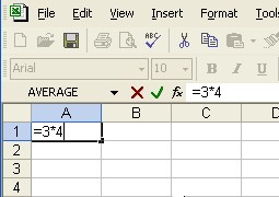
Not only can you enter data, generally as numbers or text, but you can tell Excel to perform certain calculations with that data. These calculations are entered in much the same way as data in the sense that you type them in a particular cell where you want the results to be displayed. The distinction between data, which is somewhat static (except for Excel's attempts to format it suitably), and a calculation, which requires Excel to perform some action to generate the result, is that the calculation is preceded with an "=" sign. This is the trigger that tells Excel that it needs to wake up and do something. A few other mathematical symbols (like "+" and "-") will also switch Excel into formula edit mode (causing an "=" to be inserted automatically once you hit ENTER).
 |
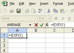 |
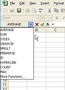
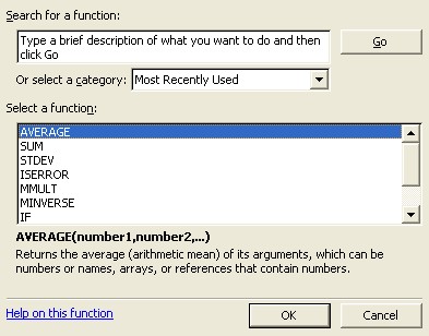
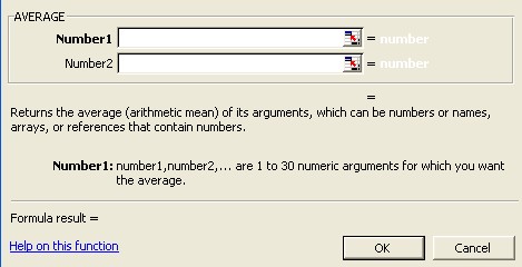
The calculations themselves may consist of basic arithmetic operations (*, /, +, -, ^, and parentheses to ensure things are done in the right order) or they may also include more complicated functions from Excel's library. These predefined functions can be inserted in the calculation in a number of different ways. First, if you already know what the function is you may type it right into the calculation. This is particularly easy with such familiar examples as =ABS(-2^2), or =1/SQRT(16). The second approach is to select from the list of recently used functions that automatically appears above the A column once you type "=" (where it says "AVERAGE" in the pictures). Finally, you may click on the little "fx" next to the formula bar to get a dialog box that presents you with the entire library of functions (arranged by categories).
 |
 |
Once you hit the ENTER key or the green check mark, the calculation you are typing is replaced with the result of the calculation. If you click once back on that cell to select it, the formula will appear in the formula bar, but not in the actual cell. If you double click on the cell with the calculation you will re-enter edit mode and the formula will reappear, both in the cell and in the formula bar.
Functions
A few words are in order about functions in general. With the exception of a few matrix/array functions (which will be discussed later), each function represents a single value (the result of the calculation the function name describes, or the "output" of the function). So, when you insert the function somewhere in the calculation, what you are doing is telling Excel to first figure out what that value is, and then replace the function with that value. Now, in order to insert the function in a calculation you must type "NAME(...)", including the parentheses. NAME represents whatever the name of the function is, like SQRT. The parentheses surround whatever information Excel needs to perform the calculation and return the correct value. The ... represents that information, referred to as the "arguments" of the function (or the "input"). For the SQRT function there is only one argument, whatever you are taking the square root of. So SQRT(16) tells Excel to take 16 as the input argument and calculate its square root, returning an output value of 4. This value of 4 is what actually gets used in any further calculations or displayed in the cell where the function was typed. Other functions, such as AVERAGE(...), may have two, three, or a whole list of arguments as input. When you select a function in the dialog box above, a new dialog is presented, prompting you for all the arguments needed. Fortunately, this dialog also provides some hints as to what those arguments represent, and even a preview of the result of the calculation.
Calculation by Address
None of this makes Excel anything more than a glorified calculator. What makes Excel truly useful is not its ability to to store columns of numbers, or even to perform individual calculations. The power of Excel lies in its ability to do lots of calculations with the numbers that you have already stored. So, rather than actually typing numbers right into the calculation or as the function arguments (as shown so far), you will instead typically refer to data that is located elsewhere in the spreadsheet. The beauty of this is that you can reuse the same calculation with different data without having to edit the function again.
 The
technique then, would be to have the input data in one location, cell
A1 for example, and have the calculation (and thus the output) in another
location. When typing in the function you would replace the input value
with the address (A1) where the input is located. This might sound unnecessarily
complicated, but it is really extremely convenient. First of all, typically
you are storing data in the spreadsheet anyway and just want to analyze
it. There is no sense duplicating all your data in the calculation.
Second, this allows you to experiment with your input data until you
produce the results you are looking for (studied in more detail later
when we talk about Goalseek). Finally, if you want to do a whole bunch
of similar calculations you don't want to have to manually type them
all or even duplicate one calculation many times and go in and edit
the input values for all of them.
The
technique then, would be to have the input data in one location, cell
A1 for example, and have the calculation (and thus the output) in another
location. When typing in the function you would replace the input value
with the address (A1) where the input is located. This might sound unnecessarily
complicated, but it is really extremely convenient. First of all, typically
you are storing data in the spreadsheet anyway and just want to analyze
it. There is no sense duplicating all your data in the calculation.
Second, this allows you to experiment with your input data until you
produce the results you are looking for (studied in more detail later
when we talk about Goalseek). Finally, if you want to do a whole bunch
of similar calculations you don't want to have to manually type them
all or even duplicate one calculation many times and go in and edit
the input values for all of them.
Calculations with Address Ranges
 Each
input argument may come from a different location if need be. In fact,
certain functions (particularly involving statistical analysis) are
specifically designed to work with whole lists of data. The most obvious
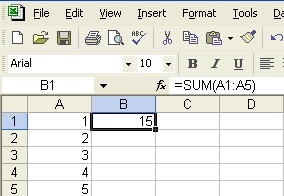
examples of these would be the SUM(...) and AVERAGE(...) functions.
Summing or averaging one number doesn't make a whole lot of sense. To
sum a whole column of numbers (typically any numbers you would want
to add up or average would be stored together anyway), you could separate
each address with commas like SUM(A1, A2, A3, A4, A5), but typing it
would be quite a chore. To get around this difficulty we use range notation.
Typing the first and last address of a contiguous range and separating
them with a colon is a shorthand way of representing a whole list of
addresses.
Each
input argument may come from a different location if need be. In fact,
certain functions (particularly involving statistical analysis) are
specifically designed to work with whole lists of data. The most obvious
examples of these would be the SUM(...) and AVERAGE(...) functions.
Summing or averaging one number doesn't make a whole lot of sense. To
sum a whole column of numbers (typically any numbers you would want
to add up or average would be stored together anyway), you could separate
each address with commas like SUM(A1, A2, A3, A4, A5), but typing it
would be quite a chore. To get around this difficulty we use range notation.
Typing the first and last address of a contiguous range and separating
them with a colon is a shorthand way of representing a whole list of
addresses.
A convenient trick when putting either addresses or address ranges in a function calculation is that, instead of manually typing in the reference (such as A1), you may take the mouse and click on the cell that you want to refer to. If you are trying to enter the notation for a range of addresses, just click down on the first cell in the range and drag the mouse over to the last one before releasing. This can sometimes mess you up if you are editing a function (either intentionally or not) and accidentally click somewhere else on the spreadsheet before hitting ENTER. You will end up with undesired references stuck in the midst of your calculation.
Auto Fill with Calculations
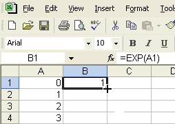
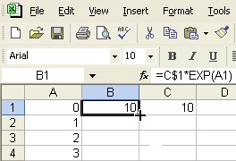
Just as you can duplicate numbers using the auto fill operation discussed on page 1, you can also duplicate calculations. However, there is little sense in repeating the same exact calculation, which is what happens if you do auto fill using actual numbers. The trick, as mentioned above, is to do calculations using addresses. The kind of address we introduced earlier is known as a "relative reference" in the sense that it will change if the formula is copied and pasted elsewhere. It will also change when duplicates are made using the auto fill operation. This is best demonstrated with a picture.
 |
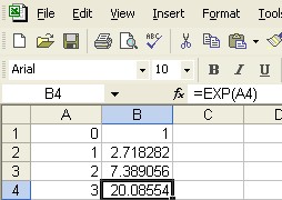 |
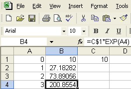
Notice that by dragging the auto fill handle down from cell B1 to B4, the calculation that started out as =EXP(A1) changed to =EXP(A4). This has the effect of generating a slightly different calculation in each row to correspond with the data (column A) in that row. In other words, the calculation continues to use data that is in the same "relative" position. If the auto fill handle was dragged horizontally instead of vertically, it would be the column label that would change (from A1 to B1, C1, D1, etc.) in order to maintain the same relative position.
Occasionally, you want to include numbers in your calculation that don't change from row to row (or column to column). This can be done by typing in the actual number, but if you want to be able to easily change this number in all the calculations it would be better to use what is called an "absolute reference". This is an address that stays the same even when you copy and paste or do an auto fill. To designate an absolute reference you precede either the row or column or both (whichever you want to remain the same) with a "$".
 |
 |
Rearranging Calculations
It was also mentioned on page 1 that selected data could be dragged to another location. This turns out to be one exception to the relative referencing. If you select a calculation and drag it somewhere else, the addresses in it won't change, they will still refer to the original data. Even better, if you select the data that is used in other calculations (doesn't matter how many) and drag it somewhere else, the calculations will be automatically updated to reflect this change in address. You can drag any data or calculations anywhere you want without being afraid of messing up your results.
Some Sample Exercises
- Label two columns by typing X and Y in the first row. In the second
row type any number you like under the X. Under the Y type in the
formula needed to calculate y = 3*x-1 referring to the address of
the value you typed under the X. Remember to precede the formula with
an "=". Your results should look something like below:
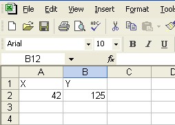
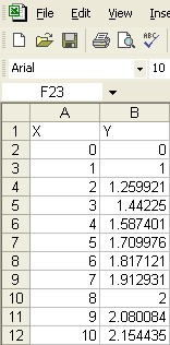
Can you manipulate the number in A2 so that the number in B2 is as close to 10 as possible? - Using the same X and Y headers as before, create two columns of
numbers. Make the first column of 11 numbers (X values) from 0 to
10 (can be done by typing in the 0 and the 1 and using auto fill to
generate the rest as in the third exercise on page 1). Make the second
column (Y values) using the function y=x^(1/3). You should only need
to type in the formula once and generate the rest of the column using
the auto fill.
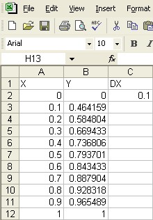
- Starting with the same data and calculations as in exercise 2, add
another column labelled DX and place a number in the cell beneath
it. The goal is to replace the value in A3 with a formula that takes
the value in the previous cell (relative reference A2) and adds the
change in X value specified by DX (absolute reference C$2). You then
select the formula in A3 and autofill the rest of the X values (but
not the first one).
Contact Leo Wibberly at ldwibber@vcu.edu or (804) 740-4650 to make appointments