| This section covers the low–level preprocessing steps from the point
at which the chip is scanned, to obtaining reliable estimates for the relative gene abundances
of each gene in all of the samples. Broadly these steps may be classified as image analysis,
quality control, background correction, and normalization; although all of these procedures are
inter–dependent, and not always done in this order. It is important to understand that
the primary goal of array image processing involves measuring the intensity of the spots, then
using this intensity measure to quantify the gene expression values. It's also important to have
a means to test and assess data reliability. A few moments will be taken to explain some basics
of digital imaging. |
| |
Basics of Digital Imaging |
| When converting any analog image to a digital image a conversion must occur.
This converstion is a combination of sampling and quantification. Sampling is the process
of taking samples or reading values at regular intervals from a continuous function. It may help to
think of an analog image as a continuous 2–dimensional function. When this analog image is scanned, say
in the horizontal direction, the variation of intensity along the horizontal direction forms a
single dimension intensity function. Scanning a 2–dimensional function, both in the horizontal direction
as well as the vertical direction (another way to say this would be; the image is being sampled),
captures a digital image, that is, a rectangular array of discrete values (see figure 1).
|
| |
Figure 1. A digital image is a 2–dimensional array of pixels.
Each pixel has an intensity value
(represented by a digital number) and a location
address (referenced by its row and column numbers).
For this figure the yellow
square is representative of one pixel. |
| Each picture element is called a pixel. This process
of converting an analog image to a digital one is called digitization.
It is not necessary to understand the details of how computer systems store images, however, one should
know a more powerful computing system will be capable of producing higher quality images. Distortions,
refered to as aliasing effects, will occur if a computing system is not capable of sampling
an analog image at the ideal rate. Another way of saying this would be; the clarity and accuracy of a
digital image depends on the abilities of the technology being used to create it.
Obviously, the best resolution possible is prefered. A general rule of thumb is to have the pixel size approximately
1/10 the size of the spot diameter. Given that the average spot diameter is at least 10 to 12 pixels,
each spot will have a hundred pixels or more in the signal area, this is usually adequate for an
appropriate statistical analysis, one which will help the segmentation. Segmentation is
the process of classifying pixels as either foreground (signal pixels) or background (this will be reviewed further
in the next section).
|
| |
Microarray Image Processing |
| As most know, a typical two-channel (two-color) microarray experiment involves two samples;
often a sample of interest and a control. These might be a disease sample and a healthy sample
or an experimentally treated sample and an untreated sample. RNA from the two samples are
reverse transcribed to obtain cDNA. The products are then labeled with
fluorescent dyes; say, red for the sample of interest and green for the control sample.
These labled cDNAs are then hybridized to the probes on the glass slides, which are in turn
scanned to produce digital images (as discussed above).
When a gene is expressed abundantly in the sample of interest and hardly at all in the healthy tissue sample
it appears as a red spot. When a gene is expressed in the control sample and not expressed in the sample
of interest, that spot appears green. When a gene is expressed in both samples it appears as a yellow spot.
Genes not expressed in either tissue sample will appear as a black spot. These possibilities are
illustrated below (see figure 2).
|
| |
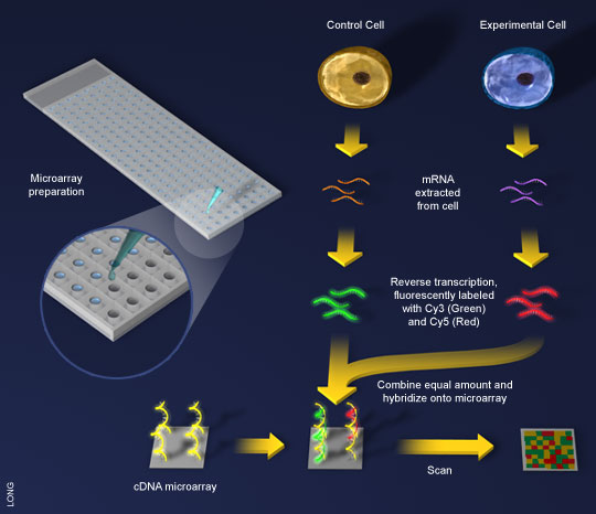
Figure 2. A general scheme for cDNA microarray. (1)mRNA is extracted from
both a control and a test cell. (2)Using reverse transcriptase, the mRNA is made into
cDNA and tagged with fluorescent colors. (3)The cDNA is exposed to the microarray,
already spotted with the genes of interest. (4)Computers scan the microarray, looking
for patterns of color. (Image courtesy of Bioteach) |
| The final product of the proccess illustrated above
(found in the lower right hand corner of the diagram) is a
sythetic image obtained by overlapping the two channels. Alot of information
can be contained in these images (see figure 3).
|
| |
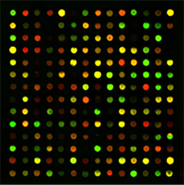
Figure 3. A two–color microarray experiment, showing
how gene expression can be altered by a disease such as cancer |
| Hybridized arrays, like the one above, are scanned to produce
high resolution tiff files. These files are then processed (with specialized software)
in order to produce quantitative intensity values of the spots and their local background
on each channel. The goal is to produce a large matrix or data frame of the expression
data; traditionally, the genes are represented by the rows, while the conditions are
represented as columns. Ultimately, through analysis and data minning one should
be able to extract biologically relavent information from the quatitative data.
|
| |
Image Quantification |
| Although the lab technician usually handles this step (using
the default settings on an image quantification program) the program and the
settings can have a noticeable impact on the noise level of the subsequent
estimates. There are several steps in image quantification: |
- Array Localization – laying the grid; finding where the printed spots ought to be in the image;
- Image Segmentation – identifying the extent of each spot, and separating foreground from background;
- Quantification – summarizing the varying brightnesses of the pixels in the foreground of each spot;
- Dealing with scanner saturation; and
- Dealing with variable backgrounds.
|
| Array Localization
|
| It would seem that Array Localization, or spot finding, would be simple
and straightforward; given that one knows in advance the number of spots, as well as their size,
and the pattern used to print them. It appears that what is needed is a program that
designates a circle of the appropriate size, while the technician scans the spots relative to the pre–set circle,
and then classifies all pixels falling within the cirlce as foreground (or signal pixels) and all the pixels falling outside
the circle as background. The technician does the first step interactively. The quantification
program must deal with several problems in the second step. It is rare that the probes are
uniform in size and shape; most programs try to adapt to the sizes, and sometimes shapes,
of individual spots. Three different methods used by programs for
addressing (griding), that is the process of identifying the location of the probes on the surface of the
microarray are: fixed circle, adaptive circle, and adaptive shape. fixed circle uses the manufacturer's diameter specifications for each spot,
all pixels within the enclosed circle are considered foreground, while all pixels
exterior to the circle are considered background. adaptive circle starts with a fixed circle diamter,
then the diamter of each spot is re–estimated using the intesities of the surrounding pixels.
adaptive shape uses spot coordinates and intensities to get the "best fitting shape"
for the spot. Sometimes (poorly stabilized) neighboring
probes bleed for some region around which may invert the relation between foreground and background (see figure 4). Three
different types of spot finding are: |
- Manual Spot Finding – This method involves computer assistance for a lab technician
who must determine the circle size for each individual spot. In the early days of microarray analysis this
was the only method, however, in the modern era of microarray spot finding this is an essentially obsolete procedure.
Clearly, this would be extremely time consuming, while introducing possible noise through human error.
- Semi-Automatic Spot Finding – This method still requires some technician assistance, however,
it is vastly superior to the Manual Spot Finding method with regards to time and labor. Algorithms are used to
automatically adjust the location of the grid lines, or individual grid points, after the approximate
location of the grid has been specified by the technician.
- Automatic Spot Finding – This method requires the least amount of time and labor on the part
of the technician. The technician would only have to provide an array configuration, that is the number of rows
and columns of spots. Once this information has been provided the processing system would search the image for
the grid position. This method elimates human error, while providing the most consistency.
|
| Image Segmentation
|
| Image Segmentation is the process of partitioning an image into a set of non–overlapping
regions whose union is the entire image. Put a different way, it is the process of classifying pixels as foreground (signal pixels)
or background. It is important to realize that only the pixel intensities determined to be foreground will be used in calculating
the signal. Pixels determined to be background are considered noise which should, of course, be eliminated.
There are several different types of segmentation: |
- Pure Spatial–Based Signal Segmentation – This is perhaps the least reliable
method of segmentation listed here. For this method two circles are used (selected by a technician
or software), one circle slightly smaller than the other. These circles will be placed
over spot locations. Software will consider any pixels inside the
smaller of the circles to be foreground, and any pixels outside the larger circle to be background (there is a limiting
square that encases both circles and the edges of this square and the larger circle dictate the area
to be counted as background). Some obvious shortcomings of this method are some spots will be smaller than the smaller circle,
causing white space to be counted as interior pixel intensity. Also, the background intensity values may be obscured
due to foriegn contaminants, or a spot whose outer diameter is greater than that of the larger circle.
- Intensity Based Segmentation – This method is more reliable than the aforementioned one, however, it too has
its shortcomings. Using a computing system with only moderate power, one may obtain results with more speed and simplicity
than other segtmentation methods. Specifically this method determines which pixels to use as signal by considering
only pixel intensity. Working from the assumption that foreground pixels will be, on average, brighter than background pixels,
the software determines the brightest 20% of the pixels for a given spot. These brightest pixels are considered foreground,
or signal pixels, while the other pixels are considered background. Spots with low intensities, or arrays with foriegn
contamination can really throw this method off, especially if exterior pixels (that should be classified as background)
are artificially bright.
- Mann–Whitney Segmentation – This method is a combination of the two mentioned previously.
Once again a circle is placed in a prep–secified target area, where a spot is known to be. Given that the pixels
outside the circle are background, one may use statistical properties (in this case Mann–Whitney) of said background
pixels in order to ascertain which foreground pixels should be used as signal pixels. A Mann–Whitney test gives
technicians an intensity level that will used to divide signal pixels from the rest. This method will determine a signal
pixel regardless of whether or not the pixels are withen the area of the spot. As always, any type of foriegn contamination
will drastically effect the technician's ability to accurately determine which pixels are signal pixels to be used for further
calculation.
- Combined Intensity–Spatial Segmentation (or the trimmed measurements approach) – This method is extremely similar
to the Mann–Whiney method. Given this similarity it will simply be mentioned here as another possible method. One may
further read about it in any microarray text.
|
| |
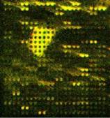
Figure 4. Some problems that quantification must deal with |
| The different programs each try different approaches to these problems,
and they make a difference in the reproducibility of gene expression measures. A study done
in California showed considerable differences among results from different quantification
programs applied to 8 arrays that compared the same two samples. Several different settings
were used on most programs. Since ratios should be identical, the standard deviation is an
(inverse) measure of quality. |
| |
| Quantification
|
| |
Figure 5. Noise levels from the same 8 cDNA slides, as
quantified in many different ways (courtesy Jean Yang, UCSF). |
| The previous figure (figure 5) shows that background subtraction added to the noise
in those measures; many researchers have had similar experience. On the other hand it
seems in principle wrong to ignore background, and some substrates (eg. poly-L lysine) show
substantial additive background; ignoring this leads to substantial bias in the estimates
of most gene ratios. At the moment there is no consensus, but two suggestions may help for
the time being. |
| It may be pragmatic to ignore the background correction, if
the goal is to detect a few differentially expressed genes among the multitude
of noisy similarly expressed genes. For this purpose noise control is most
important. On the other hand, when it comes time to estimate the fold-change, subtracting
background, or some other form of background correction gives more accurate estimates. |
| Perhaps the resolution of this paradox will come with more sophisticated
forms of background correction. The Spot program and the Agilent software both do something
different than local background estimation, and both give less noisy estimates than subtraction.
In principle the raw intensity of a spot is made up of fluorescence from labeled transcripts,
plus reflection or emission from the substrate. The label fluorescence comes from the target
transcript and also a mixture of other transcripts that have bound non–specifically to the
spot. The local background is made up of the reflection from the substrate, and stray bits
of labeled transcript that have bound to the surface (sometimes if a nearby probe has spread,
it includes labeled transcript from that other gene). The make-up of the local background
differs from the background we want to correct on the spot. On the other hand the negative
controls show just non-specific hybridization, which is the bulk of what we want to correct
on each gene probe. Perhaps a better way would be to subtract a weighted average
of the local background and the values of negative controls nearby. |
| | |