Introduction and Review

(1) r² = 1 - SSE/SST

is the proportion of the variation of Y that is accounted for by the linear relationship. Here I use the notation of the analysis of variance, where SST is the sum of squared deviations of the Y values from their mean, and SSE is the sum of squared deviations of the Y values from the values predicted by the model.When estimating the coefficients of the model from data we typically use the method of least squares, which calculates slo pe and intercept so that SSE is minimized, thus making r as large as possible. Note that the "mean squares" are important quantities: the square root of MST is the standard deviation of Y and the square root of MSE is the standard deviation of the residuals. (Unfortunately SPSS and some other statistical software mislabel the latter quantity "standard error of the estimate".)

To make the examples more concrete, suppose that Y is the freshman year GPA of students and X is their score on the Mathematics portion of the SAT. To make the arithmetic simpler, X will be measured in hundreds of points, so that it ranges from 2 to 8. Analysis of a dataset might yield the following regression equation:

(2) Y = .5 + .4 x

Sometimes a scatterplot of the two variables will indicate that the straight-line model is inadequate, and a curvilinear relationship may appear to provide much better predictions. SPSS, for instance, will find the best fitting quadratic and cubic curves and graph them on the plot. A quadratic curve has three coefficients that are estimated from the data, and there is no longer a single number that deserves to be called the "effect of X on Y". For example, a quadratic relationship might turn out to be:

(3) Y = .2 + .75 x - .04 x²

When a curve is used to describe the relationship between X and Y the Pearson correlation is not an appropriate measure of the fit of the model. Fortunately the formula given above for r²can be used, and the resulting measure (called the coefficient of determination) has the same interpretation: the proportion of variation in Y that is accounted for by the model. This generalized coefficient is always denoted by a capital R and usually presented in its squared form. SPSS calls it the "multiple R", or multiple correlation coefficient. R is always positive except in the special case of the simple straight line model, where the sign indicates the direction, upward or downward, of the line.

Using a mathematically defined curve like the quadratic rather than a straight line to express the "on the average" value of Y for each X is only one of many ways to develop models that fit the data better. In some situations it may be known that the observations (cases) fall into categories. For instance, school districts may be county or city, rural or urban, and in the example being used here the students are identifiable as male or female. On a scatterplot different symbols or colors can be used to identify the cases that belong in different categories. It is also possible to use algebra to express how predictions might be made using both the categorical variable and the original predictor X.

Indicator (Dummy) Variables as Predictors

        (4)    y = -.5 + .5 x + .5 w

The algebraic expression summarizes how to make GPA predictions, depending on the student’s SAT (value of x) and gender (value of w).

You can calculate what the predicted values of y will be for a woman with an SAT of 500 (-.5 + 2.5 +.5 = 2.5), and for a man with the same SAT (-.5 + 2.5 + 0 = 2.0). For any fixed value of x, women are predicted (according to this model) to have mean GPAs .5 points higher than the men. If you plot this equation on a graph with x as the horizontal axis and y the vertical axis you will see two parallel lines, .5 points apart vertically, with slope equal to .5 GPA points per 100 SAT points. We might refer to these coefficients as effects: the effect of being a woman rather than a man is .5 added GPA points; the effect of a hundred SAT points is .5 GPA points. But the word effect is conditional, it demands that I remember that I am "holding constant" the other independent variable in the equation.

This prediction equation is a special case of multiple regression, multiple in the sense that more than one independent variable appears in the equation. (In a sense we were already using multiple regression when talking about the quadratic curve. It too has three coefficients (including the constant term). Some people might even refer to x² as a second "independent variable", even though its value is completely determined by the value of x. A data set might even contain these squares as a separate variable in addition to the original values.) The regression procedure in SPSS simply asks for a list of names of independent variables and then uses the data to calculate the regression coefficients that will minimize SSE, the sum of squared residuals.

If you apply this model to the Freshman dataset you will find that the least squares prediction equation for this sample actually turns out to be

        (5)    y = 1.045 + .255 x + .197 w

Holding SAT (x) constant, women would be predicted to be about .20 GPA points higher than men on the average. Furthermore, students of the same sex who differed by 100 SAT points would be predicted to differ by about .25 GPA points. T-tests provided by SPSS indicate that both of these "effect" coefficients have P-values below .10. The coefficient of w, however, has a two-sided P-value of .07, which might not be judged significantly different from zero by some.

The R² for the prediction equation is .077. This is slightly larger than the value obtained by using a simple straight line without identifying the students’ sex (.064).

Interpreted geometrically, the equation with two predictors can be plotted as two parallel straight lines, one fitted to the men’s scores and the other to the women’s. The equations of these two lines are:

        (6)     Men: y = 1.045 + .255 x
            Women: y = 1.242 + .255 x

Algebraically, we can use one "complex" equation for prediction or two "simple" equations! Either formalize the separation of the sample into two groups by introducing the indicator variable w or just verbalize the distinction between "men" and "women."

Different Slopes for Different Folks (Interaction)

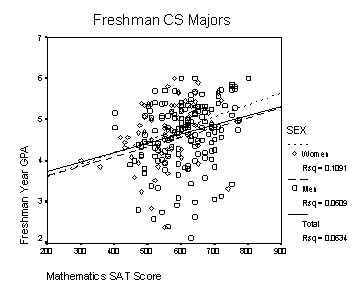
When we plot these data using the SPSS scatterplot procedure with a "marker" identifying the sex of each person, we are allowed to fit straight lines separately to the two groups. These lines are not parallel, of course: both the slope and the intercept are separately estimated in each group. I can use the "Split File" command in SPSS to find the equations of these lines. They are:

        (7)  Men:    y = 1.158 + .237 x
            Women: y = 1.146 + .290 x

These lines diverge as the SATM score x increases, as the effect of a 100 SAT point difference adds .29 to women’s predicted GPA but only .24 to men’s. Note the different interpretation of this model compared with the previous (parallel line) one: women do not simply have higher GPAs at every level of SATM. At the lowest level of SATM (200) the predicted values of GPA are about the same for men and women, but the gap increases as the scores increase.

Previously I showed the equivalence of a complex equation to two simple equations. The same thing can be done in reverse with this model. We need to define another predictor variable, this time the product of w and x. Let v = wx. The equation

        (8)    y = 1.158 - .012 w + .237 x + .053 v

makes exactly the same predictions as the previous two straight lines do. The coefficients of w and v are differences: the differences between the male and female intercept and slope, respectively.

In the statistical literature the product of two predictors is called an interaction variable, and if its regression coefficient is significantly different from zero the predictors are said to have an interaction effect on the dependent variable.

The Reading Experiment: One way ANOVA

Multiple regression with the variables s and d as predictors (independent variables) and pre1, the value of PRE1 (pretest number 1) gives the equation:

        (9)    pre1 = 10.50 - .77 d - 1.36 s .

This equation predicts an average score of 10.50 if both d and s equal zero. It is not a coincidence that 10.5 is the mean PRE1 score for the children in the Basal class, i.e., for the children with zero values on both d and s. The other regression coefficients are the differences between the Basal mean and the other group means. This multiple regression equation "predicts", in fact, the exact values of the three group means. Once again it is possible to see why people like to call these regression coefficients "effects": the effect of being placed in the DRTA group rather than in the Basal group is, on the average, -0.77 points. In more descriptive terms, the children in the DRTA class scored .77 points lower than the children in the Basal group.

Of course, since the pretest was given before any instruction had taken place, it is incorrect to think of -0.77 as the effect of the instructional method DRTA on these scores! The difference may be due to a failure of the randomization process (if indeed randomization took place), or it may have something to do with the way the pretest was administered. (Note: neither of these regression coefficients is significantly different from zero at the .05 level!) It is more appropriate to speak of effects when a posttest variable is examined the same way. For example when the dependent variable is the first posttest, POST1, the multiple regression program tells us that

(10)     post1 = 6.68 + 3.09 d + 1.09 s .

Both experimental classes did better, on the average than the Basal group, which averaged 6.68 points on post1. The DRTA group did 3.09 points better, the Strat group only 1.09 points better. (Verify from your previous research that the last two numbers were the mean differences between Basal children and the DRTA and Strat children, respectively.)

Including a Covariate in the Model: ANCOVA

        (11)    post1 = -.60 + 3.62 d + 2.04 s + .69 pre1

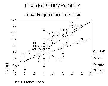
From our previous discussion it should be clear that if a graph of this relationship is drawn using pre1 as the X axis and post1 as the Y axis, we will have 3 straight lines. They are parallel, with slope .69. One line describes predictions about the Basal class, where d = s = 0 ; one to the Strat class, where d = 0 and s = 1; and the third about the DRTA class, where d = 1 and s = 0. (Exercise: write down the equations of the three lines in the usual algebraic style.)

Once again consider the meaning of the coefficients of d and s in the last two equations: the effect of being in the specified class rather than in the Basal class, holding constant pretest score. Earlier we called 3.09 the effect of being assigned to the DRTA class rather than to the Basal class; now the effect is 3.62 points. The latter is properly interpreted as conditional on the value of PRE1. If we compare children who scored the same on the pretest, we should predict that on the average the ones in the DRTA class will score 3.62 points higher on the Posttest than the children in the Basal class. And the slope of the line? The coefficient of pre1? It is the difference in average score of children who differ by one point on the pretest, assuming that they are all in the same class. Sometimes this is abbreviated to "the effect of a one point difference in pre1, holding constant the treatment."

Interaction Effects in ANCOVA

        (12)    post1 = 1.79 + 1.31 d - 2.02 s + .47 pre1 + .22 id + .41 is

Rewriting this in the form of three straight lines, so that it can be interpreted more easily, the prediction model becomes:

        (13)   Basal: post1 = 1.79 + .47 pre1
                    DRTA: post1 = 3.10 + .69 pre1
                     Strat: post1 = - .23 + .88 pre1

It may help a bit to see the three lines plotted.

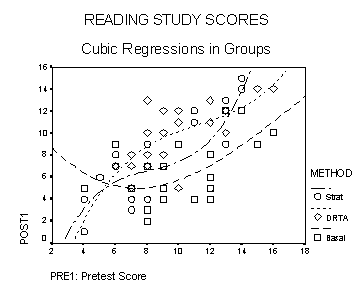
While we are at it, we might as well record what happens when we ask for quadratic or cubic functions (curves) to be fit separately to each class of children. Each of those plots can be translated into a single prediction equation that involves the indicator variables d and s ! One important point: while the graphs yield obviously different predictions when extrapolating from extremely large or small values of pre1, the predictions made in the central portion of the graphs (say between pretest scores of 6 and 13) are not that different.

Here are some explanations of terms that you will come across in advanced applications of regression modelling and analysis of variance. Some come up in Agresti & Finlay's Chapter 11, others can be found in Chapters 12, 13, and 14.

• Adjusted R square is defined as 1 - MSE/MST . Notice the resemblance to the definition of R square. If the sample size is very large compared with the number of variables in the equation these two quantities will be nearly identical, since the degrees of freedom total will be very close to the error degrees of freedom. An interesting property of adjusted R square is that it will continue to increase as long as there is a predictor variable available whose regression coefficient has a t-ratio that is bigger than 1.00.
• Beta weight, or what SPSS refers to as Beta in its output, is a standardized regression coefficient. These coefficients are what you would get if all the variables had been standardized, converted to Z-scores by subtracting the mean and dividing by the standard deviation, before doing the regression analysis. Thus, if beta = .40 , we would expect that a difference of 1 standard deviation on X would be associated with a .40 standard difference in Y on the average, holding constant the other predictors in the model. Researchers who use variables that have no clearcut scale of measurement tend to prefer to report betas, while folks in the policy sciences who deal with test scores, ages, dollars and the like prefer to use unstandardized coefficients in their reports.
• Effect is sometimes used to describe a regression coefficient, as illustrated in my discussion of Equation (5) in part 1 of these Notes. It suggests a causal interpretation of the relationship. Sometimes it just doesn’t make sense when taken literally: take Equation (3) for example. In that quadratic equation neither regression coefficient is an "effect"; as I noted, the real effect of x varies as x changes.
• Main Effect is a term used in two-way (or "multi-way") ANOVA. In these analyses the subjects are divided into groups, but there is an obvious structure to the classifications. For example, children may be randomly assigned to reading classes that use different teaching methods, but some classes may meet in the morning and others in the afternoon. The researcher may want to know whether the instructional method has "an effect" compared to other methods, but also whether the time of day has an effect. In terminology that I hope will become more fashionable, main effects can be thought of as contrasts with respect to the oneway ANOVA on all classes.

Extending the reading study, for instance, suppose there were 6 classes: morning classes BM, SM, DM and afternoon classes labeled BA, SA, and DA. The existence of a main effect for time of day would be tested by examining the contrast 1/3(sum of the first three class means) - 1/3 (sum of the second three means). The main effect for method, however, is more complicated since there are 3 methods used.
• A Two-way or Multi-way ANOVA can always be carried out as a regression analysis with indicator (dummy) variables. Thus M. Hardy’s Model 3 (p. 20) can be thought of as a 2-way, 2x6 ANOVA problem, since Race has two categories and Occupation has 6 categories. The complex null hypothesis that "Occupation has no effect on Income, controlling for Race" specifies that the true value of the 5 OCC coefficients in Model 3 are zero. In ANOVA jargon, one might say the hypothesis is that there is no main effect of Occupation. This main effect is tested by comparing the SSE of Model 3 with the SSE of Model 1, or equivalently, by asking whether the increase in R square is significantly different from zero. (See Hardy, p. 22.) (See also Expanded ANOVA Tables below.)
• Interaction Effects occur when the effect of one predictor depends on the value of a second predictor. For example, in the reading example, suppose that in the morning classes the Strat students did better than the DRTA students but in the afternoon classes the situation was reversed. We’d say that method interacts with time of day in its effect on learning. In regression models interaction effects are represented by products of indicator variables. See my comment on Equation (8) above. Note also Hardy’s Section 4, and her use of product variables in Model 5 (page 33): "The new variables, BLOCC . . . are computed by multiplying BLACK with each of the occupational dummy variables."
• Covariance Analysis or ANCOVA refers to an analysis in which there are both categorical ("qualitative") and quantitative predictor variables. Usually at least on of the categorical variables will be the causal variable of interest, and we are primarily interested in its effect on Y conditional on the other variables. Hardy’s example is a good one: the issue is whether there exists salary discrimination against blacks. The other variables, such as occupational class, education, time on the job, etc., are introduced as control variables or co-variables to see if the initial difference in mean income holds up. The format of an ANOCOA presentation will usually emphasize the significance (or non-significance) of the main effect for the causal variable. While Hardy’s Table 3.3, showing all the estimated regression coefficients and their standard errors, is the standard way to present a multiple regression, an ANCOVA presentation might have simply noted that the coefficient for BLACK (the "effect of race" might be the phrase used by the researcher) was highly significant (t = -7.01) . The effects of the other variables would not be interesting, just as in my extension of the reading study time of day is considered just a nuisance. Yes, it affects learning, and thus should be controlled for, but "we" are interested in the things we can manipulate, and collect royalties from, like type of teaching method.
• F-statistics are sometimes related to t-statistics. Anytime an F has just one degree of freedom for its "numerator degrees of freedom" it is precisely equal to the square of a t with the same degrees of freedom as the denominator of the F. You’ll come across articles where someone will use F where you might expect a t, or vice versa.
• Expanded ANOVA tables can include more than the two lines for "model" and "error" (or "between groups" and "within groups"). Consider the Freshman dataset. If we use all three high school grades and both SAT scores as predictors of GPA the SSE is 106.8 (the total sum of squares, SST, is 125.4). If only the three high school grades are used the SSE is 107.8. Thus, by adding two more predictors (using two degrees of freedom), we have explained 107.8 - 106.8 = 1 more of the TSS. This can be summarized in the following ANOVA table, based on M&M’s Figures 9.21 and 9.25:

Source   Sum of Squares  df  Mean Square    F

3 HS Grades   27.71       3     9.237    18.85
2 SAT Scores   0.93       2     0.465     0.95
Residual     106.82     218     0.490
TOTAL        135.46     223

The second F statistic, .95 = .465/.49, is not significant, demonstrating that adding the SAT scores to a model that already includes high school grades does not improve the R square of the model significantly. In Hardy’s Table 3.3 (page 27) the line labeled F (change) contains a number calculated according to the same procedures as this value of F = .95 .

Reference:
Hardy, Melissa A. (1993). Regression with Dummy Variables. Sage University Papers, QASS # 07-093, Newbury Park CA: Sage.

Corrected April 8, 2003
Neil W. Henry

Virginia Commonwealth University