Figure 1. A quantile plot |
| A drawback of the t-statistic for microarray
datasets is that most experiments have only a few samples in each group (n1 and
n2 are small), and so the standard error si is not very reliable. In
a modest fraction of cases, si is (by normal sampling variation)
greatly under-estimated, and genes that are little changed give rise to extreme
t-values, and therefore false positives. The theory compensate for some of
these false positives, in that the tails of the t-distribution are much further
out than those of a Normal curve. This causes a reverse problem: a truly
changed gene has to change a great deal to give convincing evidence; therefore
many of the moderately changed genes won’t show convincing evidence of change. |
| Tusher and Tibshirani suggested (a form of) the
following test statistic t* rather than the usual t statistic[1]. The SE in the
denominator is adjusted toward a common value for all genes; this prevents gross
underestimation of SE’s, and so eliminates from the gene list those genes that
change only a little: |
| t* = (xi,1 – xi,2)
/ ((si + s0)/2) |
| where s0 is the median of the
distribution of standard errors for all genes. The range of values of the
revised denominator is narrower than the range of sample SEs; it is as if all
the SE’s are ‘shrunk’ toward the common value s0. Unfortunately no
theoretical distribution is known for this statistic t*, and hence the
significance levels of this statistic must be computed by a permutation method
(see below). A similar statistic also crops up in empirical Bayes analysis (see
below). |
| Another approach to detecting more of the
differentially expressed genes is to use a more precise estimate of the
variation between individuals, for each gene, in tests of that gene. If a good
deal of prior data exist on the tissue and strain used in the wild-type (or
control) group, measured on the same microarray platform – and this is
sometimes the case now – then it is defensible to pool the estimates of wild-type
variation from each of the prior studies, and use this as the denominator in
the t-scores. The t-scores should then be compared to the t-distribution on a
number of degrees of freedom, equal to that used in computing the pooled
standard error. A variant of this approach may be used in a study where many
groups are compared in parallel. The within-group variances for each gene may
be pooled across the different groups to obtain a more accurate estimate of
variation. This presumes that treatments applied to different groups affect
mostly the mean expression levels, and not the variation among individuals. Of
course one should test that the discrepancies in variance estimates are not too
large for many of the genes that are selected as differentially expressed. This
may be done by computing the ratios of variances between groups (F-ratios), and
comparing to an F-distribution. |
| Since gene expression values are not
distributed according to a Normal curve, some researchers have used
non-parametric tests. The most commonly used test of this type is the Wilcoxon
signed-rank test. Unfortunately this is not really a good choice, because the
Wilcoxon test assumes that the distribution of the gene expression values,
although not Normal, is strictly symmetric; the p-values from this test are
inaccurate, if this assumption is badly wrong; and in practice the distribution
of values of a single gene is frequently quite asymmetric. A thoroughly robust
non-parametric test is the rank, or binomial test, which counts the number of
values in each group greater than the median value, and compares this number to
the binomial distribution. This test has very little power to detect
differences in small groups, which are typical of microarray studies, and is
never used in practice to detect differential expression. |
| Gene expression values don’t follow a normal
curve, but the p-values from a standard t-test aren’t far away from truth when
the distribution is moderately asymmetric. However the t-test does fall down
badly when there are outliers (values more than twice as far from the mean as
all the others). For this reason, when doing a t-test, it is wise to confirm
that neither group contains outliers. In practice, it often happens that genes
detected as different between groups, are actually expressed very highly in
only one individual of the higher group. Some methods for doing this
pre-analysis are discussed in the Exploratory Analysis section. Probably the
best way to avoid the problem with outliers is to use robust estimates of mean
(trimmed mean) and variability (mean absolute deviation). However no
theoretical distribution is known for these; and their significance levels
(p-values) would have to be computed by permutations. |
| |
Permutation Tests |
| Permutation testing is an approach that is
widely applicable and copes with distributions that are far from Normal; this
approach is particularly useful for microarray studies because it can be easily
adapted to estimate significance levels for many genes in parallel. The major
drawback for experimentalists is that these tests usually require some
programming. Some recent software packages, notably SAM, implement permutation
testing in a menu-driven interface. |
| The meaning of a p-value from a permutation
procedure differs from the meaning of a model-based p-value. The model-based
p-value is the probability of the test statistic, assuming that the gene levels
in both the treatment and control groups follow the model (eg. a Normal
distribution). A permutation-based p-value tells how rare that test statistic
is, among all the random partitions of the actual samples into pseudo-treatment
and pseudo-control groups. The steps in a permutation-based computation of the
significance level of a test statistic are as follows: |
- Choose a test statistic, eg. a t-score for a comparison of two groups,
- Compute the test statistic for the gene of interest,
- Permute the labels on samples at random, and re-compute the test statistic for the
rearranged labels; repeat for a large number (perhaps 1,000) permutations, and finally,
- Compute the fraction of cases in
which the test statistics from iii) exceed the real test statistic from ii).
| The p-value
for the gene is the fraction of cases in which the randomly permuted samples
give a test statistic for that gene, at least as extreme as the one that occurs
in the properly labelled samples. The idea is that if the gene is distributed
similarly in both treatment and control groups, then the difference statistic
(a t-statistic or any other) will appear about as big in the permuted
arrangement, as in the true arrangement. If the gene levels in the treatment
group are higher than any levels in the control group, then no value of the
permuted statistic will be as great as the true value. |
| A permutation
test needs at least two groups of six samples, in order to have enough
different permutations. For two groups of six, there are C(12,6) = 924 permutations that give
different groups; although half of these permutations are mirror images of the
other half, so the true number of distinct pseudo-scores is 462. Some
statisticians use balanced permutations: where each pseudo-group has roughly
equal representation from both the true treatment and the true control group.
The true test statistics typically stand out better from this group of permutations,
giving more extreme p-values, but at the cost of requiring larger numbers of
samples; for example for two groups of six there are only C(6,3)2 /2
= 200 distinct balanced pseudo-groupings. |
| |
Volcano Plot |
| However one chooses to compute the significance
values (p-values) of the genes, it is interesting to compare the size of the
fold change to the statistical significance level. The ‘volcano plot’ arrange
genes along dimensions of biological and statistical significance. The first (horizontal)
dimension is the fold change between the two groups (on a log scale, so that up and down
regulation appear symmetric), and the second (vertical) axis represents the
p-value for a t-test of differences between samples (most conveniently on a
negative log scale – so smaller p-values appear higher up). The first axis
indicates biological impact of the change; the second indicates the statistical
evidence, or reliability of the change. The researcher can then make judgements
about the most promising candidates for follow-up studies, by trading off both
these criteria by eye. With a good interactive program, it is possible to attach names to genes that appear promising. |
| |
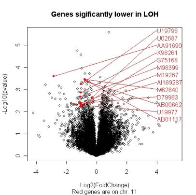
Figure 2. A volcano plot |
Genome-Wide Comparisons, Corrected P-Values, and False Discovery Rates |
P-Values and False Discovery Rates |
| Most scientific papers quote p-values, however
few papers discuss their meaning. In order to understand what the problem is
with quoting p-values for massively parallel comparisons, we need to be
precise. Let’s consider, for example, a t-test of differences between two
samples. If there is no systematic (real, reproducible) difference between
groups, nevertheless the t-score for differences between groups is never
exactly 0. Common sense cannot decide whether a particular value provides
strong evidence for a real difference. The natural question to ask is: how
often a random sampling of a single group would produce a t value as far from 0
as the t we observed. When you declare an effect is significant at 5%, you say
you are willing to let one false positive sneak in, roughly every twenty tests.
We don’t accept this for critical decisions; we won’t long continue to cross
the street, if we do so on a 95% confidence that there is a break in traffic.
We may call this the false positive rate (FPR); the FPR of a procedure is the
fraction of truly unchanged genes which appear as (false) positives. |
| If the aim of the microarray study is to select
a few genes for more precise study, then the goal is an ordered list of genes,
most of which are really different (true positives). Another way to say this is
that the expected number of false positives is some reasonable fraction (for
example less than .3) of the genes selected. This goal leads naturally to
specifying the false discovery rate (FDR) for a list, rather than significance
level (FPR). The FDR is the expected fraction of false positives in a list of
genes selected following a particular statistical procedure. For example, doing
a t-test on all genes, and selecting those whose t-score is above a threshold
of the .05-point of the t-distribution would be such a procedure. If following
this procedure in many experiments would give gene lists including twenty per
cent false positives, on average, then the procedure's FDR is 20%. The FDR is
distinct from the false positive rate (FPR), which is the rate at which truly
unchanged genes appear as false positives. If following a particular
statistical procedure on samples with no (really) changed genes gives one
positive (falsely) in every fifth experiment, then the procedure's FPR is 20%. |
| Related to the FDR is the q-value, introduced
by Storey [2]. The q-value is the smallest FDR at
which a particular gene would just stay on the list of positives. This is not
identical to the p-value, which is the smallest false positive rate (FPR) at
which the gene appears positive. The p-value is much stricter than the q-value. Most of
the researchers, who compute significance of genes by permutations, are actually computing
the q-value, rather than the p-value. |
| As of yet no conventions have been established
for false discovery rate in published work. An FDR of 5 or 10% should be
acceptable for journal publication of gene lists, in keeping with the practice
of accepting 5% of erroneous single results. For individual follow-up
experiments, the investigator must decide what's an acceptable waste of time.
If the investigator is selecting only half of the genes for follow-up based on
a priori biological plausibility, then perhaps a less stringent criterion is
acceptable. |
Multiple Testing P-Values and False Positives |
| Suppose you compare two groups of samples drawn
from the same larger group, using a chip with 10,000 genes on it. On average
500 genes will appear ‘significantly different’ at a 5% threshold. For these genes,
the variation between samples will be large relative to the variation within
groups due to random, but uneven allocation of the expression values to the
treatment and control groups. Therefore the p-value appropriate to a single
test situation is inappropriate to presenting evidence for a set of changed
genes. |
| The quantile plot can single out a modest
number of genes that are really different, but it is not a rigorous or
systematic procedure, and can’t really handle large numbers of differentially
regulated genes. Statisticians have devised several procedures for adjusting
p-values to correct for the multiple comparisons problem. The oldest is the
Bonferroni correction; this is available as an option in many microarray
software packages. The corrected p-value, pi* for gene i
is set to: pi* = Npi, if Npi
< 1, or 1, if Npi > 1; where pi is
the p-value for a single test of gene i, and N is the number of genes
being tested (which may be less than the number of genes on the array). This is
correct, but too conservative. In practice, few genes meet this strict
criterion, including many, which are known differentially expressed from other
work. Some researchers use a related ‘single-step’ adjustment procedure: they
find the smallest p-value, p(1), which is corrected to Np(1);
then the next smallest p-value p(2) is corrected to (N-1)p(2),
unless this is smaller than Np(1), in which case it is
corrected to the identical value Np(1); successively larger
p-values are corrected in similar fashion. This procedure is still too
conservative; in fact since N is usually over 10,000, and the number of
genes is a few hundred, this procedure gives corrected p-values that are almost
the same as the Bonferroni. The reason that both these procedures are too
conservative is that test statistics are correlated. |
| To give some idea of why correlation makes a
difference, imagine an extreme case: suppose all genes are perfectly
correlated, and not changed between groups. In that case the tests for all the
genes give identical results: the p-values for one gene are the p-values for
all. In this case no correction for multiple-comparisons is needed, because all
the t-scores either exceed or fall short of the threshold together. For
example, if the researcher sets a threshold at the 5% point, then no genes will
appear as (false) positives in 95% of all experiments testing for differential
expression. Of course, when false positives occur, a great number occur: in 5%
of all experiments, all genes will appear as (false) positives; the false positives
are ‘clumped’. In practice real gene expression levels are highly correlated,
because genes are co-regulated; hence the probability of false positives is
much less than calculated by the Bonferroni procedure; on the other hand, when
false positives do occur, they tend to occur in abundance. The number of
extreme test statistics, and therefore apparently significant p-values, for
correlated genes will be more variable than for independent genes, although it
will have the same long-run average. Therefore for realistically correlated
data, the multiple testing correction of p-values should be weaker than the
correction for independent genes. For example, suppose repeated experiments are
done with the two groups drawn repeatedly from the same cell line; suppose that
2% of the (unchanged) genes appear significant at the .05 threshold, in 90% of
the experiments, and 40% of the genes appear significant at the .05 threshold,
in 10% of experiments. Suppose we adopt a procedure of selecting
‘differentially expressed’ genes, only if more than 2% of the genes
individually appear significant at the .05 threshold; this procedure will
select false positives only in 10% of the experiments. That is, the corrected
p-value for more than 2% genes at the .05 level, should be 0.10 (10%). |
| This gives us an approach to correcting for
multiple testing: for a group of genes, which appear to differ between sample
types, we ask how often would a group this size exceed the threshold that these
genes exceed? To be precise: for a specific number k and a threshold α,
how often will random sampling
from the same group give at least k single test p-values will fall under
the threshold for significance level α? In practice we don’t have the
luxury of repeating experiments that
could give us these estimates. However we can calculate the results of an
experiment, where we resample from our existing samples, and calculate how
often large groups of genes appear significant. |
Calculating Permutation-Based Corrected P-values |
| To calculate corrected p-values, first
calculate single-step p-values for all genes: p1, …, pN.
Then order the p-values: p(1), …, p(N),
from least to greatest. Next permute the sample labels at random, and compute the
test statistics for all genes between the two (randomized) groups. For each
position k, keep track of how often you get at least one p-value more
significant than p(k), from gene k, or from any of the
genes further down on the list: k+1, k+2, …, N. ?After all
permutations, compute the fraction of permutations with at least one apparently
more significant p-value less than p(k). This is the
corrected p-value for gene k. Although this procedure is complicated, it
is much more powerful than the other corrections: that is, the procedure gives
a much smaller corrected p-value for each gene than the Bonferroni procedure,
and therefore a bigger list of significant genes at any corrected significance
level (specified risk of false positives). This is known as the Westfall–Young
correction <refs>. |
| There is a related procedure for computing
false discovery rates in the presence of correlation. The FDR procedure is
simpler, however it is still under some debate. When this debate is resolved,
computing an FDR may be the best way to indicate degree of evidence within the
traditions of classical statistics. However there are several emerging
approaches from the tradition of Bayesian statistics, which seem even more
powerful. |
Empirical Bayes Methods |
| Bayesian approaches make assumptions about the
parameters to be estimated (such as the differences between gene levels in
treatment and control groups); used intelligently these assumptions can make
use of prior experience with microarray data. A pure Bayes approach assumes specific
distributions (prior distributions) for the mean differences of gene levels,
and their standard deviations. The empirical Bayes approach assumes less,
usually that the form of these distributions is known; the parameters of the
prior distribution are estimated from data. As we get more detailed knowledge
of the variability of individual genes, it should become possible to make
detailed useful prior estimates based on past experience. A simple empirical
Bayes approach to identifying changed genes runs as follows, in two stages. |
| We
believe that all unchanged genes have a range of variances that follow a known
prior distribution. We estimate the mean of that distribution as the mean of
the experimental variances for all the genes. We estimate the variance of that
distribution as the variance of the gene variances. Both of these estimates
assume that a small minority of genes are actually changed. Then we consider
each gene individually. We would like an estimate of the variability of that
gene that is more reliable than its’ sample standard deviation. One way to
derive that is to work backward from the assumption that the gene variances
follow the known distribution. We can compute the probability of any value for
sample variance, given a supposed value for the (unknown) true variance of that
gene. If we combine that with the prior assignment of probability for each true
variance of a gene, we can work out the probabilities that various possible
true values underlie the one observed value of the variance. Not surprisingly
it is more probable that a very high sample variance comes about by an
over-estimate of a moderately high variance, than a true estimate of a very
high variance, simply because there are many more moderate variances than high
variances, and over-estimates are not very uncommon compared to precise
estimates. In the Bayesian tradition we construct a density function for the
probability function for the true value of the gene variance (called a
posterior distribution). To come up with a single value we might estimate the
expected value of the posterior distribution. By considerable algebra, this
expected value turns out to be a weighted average of the sample variance for
the gene, and the mean of the prior distribution, which was set to the mean of
all the sample variances. Thus we can obtain a theoretically more reliable
estimate of variation, by pooling information about variation, derived from all
genes simultaneously. This more reliable estimate of variation should then
translate into more reliable t-scores, with more power to pick up moderate
differences in gene abundance between samples. |
| In practice this works not badly at all. The
empirical Bayes estimate of variance is closer to the mean variance, more often
than the sample variance, which means that the moderated t-score is more likely
to have a moderate (not very small, not very large) value than a true t-score.
However the tails of the moderated t distribution are fairly close to the tails
of a t distribution based on a more reliable variance estimate, that is, with a
higher number of degrees of freedom. This means that a given difference in
means often gives a more significant p-value, and that more genes are selected
at a particular threshold. However there is more possible, again if we are
willing to make another fairly precise assumption. |
| The second stage of the empirical Bayes
procedure is to use prior beliefs about the number of genes that will be
changed. Suppose that based on past experience we believe that some fraction p1
of genes are actually changed by the treatment, and the remaining fraction p0 =
1 - p1 are unchanged. Then we examine the distribution of the p-values from all
the t-scores from all the genes in the experiment (not just the significant
ones). This is better done with the raw (rather than moderated) t-scores, since
the distribution of moderated t-scores doesn’t quite match near 0, where the
larger p-values are. The way that p-values are constructed for a t-score, we
should find even numbers of p-values in any interval of the same length. We
find generally that there are fewer p-values in the range 0.5 to 1.0 than there
should be (there should be N/2 such p-values), and correspondingly more in the
range 0.0 to 0.5. The natural assumption is that some genes are missing from
the range 0.5 to 1.0, because they are really differentially expressed. The
number of genes remaining, out of the total N/2 that we would expect, gives an
estimate of p0, the fraction of genes that are unchanged. Let's look at the
fraction of p-values between .5 and 1, say M. Then p0 ≈ M/(2*N). |
| Once we have prior empirical estimates of p1
and p0, we can construct the odds ratio for change in expression versus
unchanged; that is, we can estimate the probability of getting any particular
t-score if the gene is changed, and compare that to the probability if the gene
is unchanged. The ratio of probabilities is the odds, and we imagine placing a
bet on those genes with odds ratios in favor of change, above a particular
threshold. The probability of getting a particular t-score from an unchanged
distribution is the t-distribution. The probability of a particular t-score
given a changed gene depends on the magnitude of the change. This would be easy
to work out, if say we were interested only in genes with a two-fold or greater
change. Then the probability distribution can be worked out. If we want to
detect genes of any change, then we need to specify a prior distribution for
the size of the fold-changes among genes. This is very difficult to estimate empirically. |
| Another approach to this does away with the
assumption of a specific fold change in the changed genes, at the cost of
considerably increased complexity. The distribution of t-scores from the
unchanged genes is of course a t-distribution. The distribution of t-scores
from changed genes is some other unknown distribution, presumably with wider
tails, and possibly bimodal (see figure). The distribution of all scores is the
mixture of these two distributions with mixture parameters p0, p1.
The density function of all the t-scores is p0f0(t) + p1f1(t).
Then for a given gene with t-score ti, the posterior probability of
belonging to class 1, is given by Bayes' formula: P(1|t) = P(t & 1) / P(t)
= p1f1(t) / f(t) = 1 - p0f0(t)/f(t),
where f0 is the known t-distribution and f is the empirical
distribution. In practice this is reasonably robust provided that the tails of
f are fairly thick, and that a well-conditioned estimate for the density is
used. It's best to fit the distribution function with a smooth curve and take a
first derivative, insisting that it be monotone. |
Several Groups – Analysis of Variance |
| Many current microarray studies compare more
than two groups. Sometimes the question is to determine differences among three
or more cell lines, or strains of experimental animal. Another common design
compares the effect of a particular treatment (often a ligand for a receptor),
on cell lines (or animals) with wild-type and mutant versions of the receptor.
Usually the experimenter wants to know which genes are actively regulated
during treatment in both cell lines, or wants some criterion for selecting
those that are differentially regulated among groups. These questions belong in
the tradition of analysis of variance (ANOVA). |
| Generally, all of the procedures that were
discussed above in the context of two-sample comparisons, carry over to
analogues in ANOVA. However the ANOVA analogues are more complex, because many
hypotheses are being tested, and some nested within others. Especially in the
factorial design case, there is no obvious way to do permutation testing to
obtain genome-wide p-values for the interaction (2nd order) effects.
Several researchers have suggested permuting the residuals from a fit of the
main effects to obtain a permutation distribution. |
| Analysis
of variance is complex and many researchers don’t bother; they do t-tests on
the contrasts that interest them. This procedure is less effective than
analysis of variance for two reasons. The power of a t-test to pick up a
difference increases with greater confidence in the denominator – the estimate
of variability. ANOVA computes a consensus estimate of variability within
groups, based on all the groups. This estimate, based on more information, has
more confidence (greater degrees of freedom) than the variability estimated
between two samples alone. Thus for the same degree of difference, and the same
variability estimate, the ANOVA will pick up more differences than the t-test.
It’s possible to use the consensus estimate of variability in the t-score
denominators for all tests. |
| Sometimes
when researchers compare treatment effects on WT and mutant, they look for
genes that are significant on one list and not on the other. This procedure is
very fallible; if genes are changed by treatment to the same extent in both
samples, according to statistical theory, the significance levels should
fluctuate considerably. Many should appear on one list but not on the other.
The ANOVA for a factorial design is the most efficient way of identifying the
true changes in regulation under treatment among the many noisy genes. |
| |
| |
| 1. Tusher,
V.G., R. Tibshirani, and G. Chu, Significance
analysis of microarrays applied to the ionizing radiation response. Proc
Natl Acad Sci U S A, 2001. 98(9): p.5116-21. |
| 2. Storey,
J.D. and R. Tibshirani, Statistical
significance for genomewide studies. Proc Natl Acad Sci U S A, 2003. 100
(16): p. 9440-5. |
| | |