The simplest example of chaotic dynamics arises in the case of the logistic equation which has the following motivation. Imagine a growth process in ecology, economics, or some other related growth process. The system is monitored in discrete time steps, e. g. generations, years, etc. Let X_n represent the population size in the nth generation. The most naive growth law would be that the next generation depends on this one in a proportional way, with the growth factor, r, a being the constant of proportionality.

A somewhat more sophisticated model says that, if unchecked, the growth will follow an exponential law,

If r > 1 , X tends towards infinity.

A more realistic model recognizes that growth is limited by limited resources, space,etc and that these impediments also increase with population. As X_n tends to get large, the growth rate tends to slow down. The simplest way to incorporate this is to let r = A(1-X_n). Then the expression is

With this model one can calculate the growth of this population on a hand calculator. If you try it, you must supply a numerical value of the growth parameter, A, and some initial population size, X_n (0 < X_n < 1).

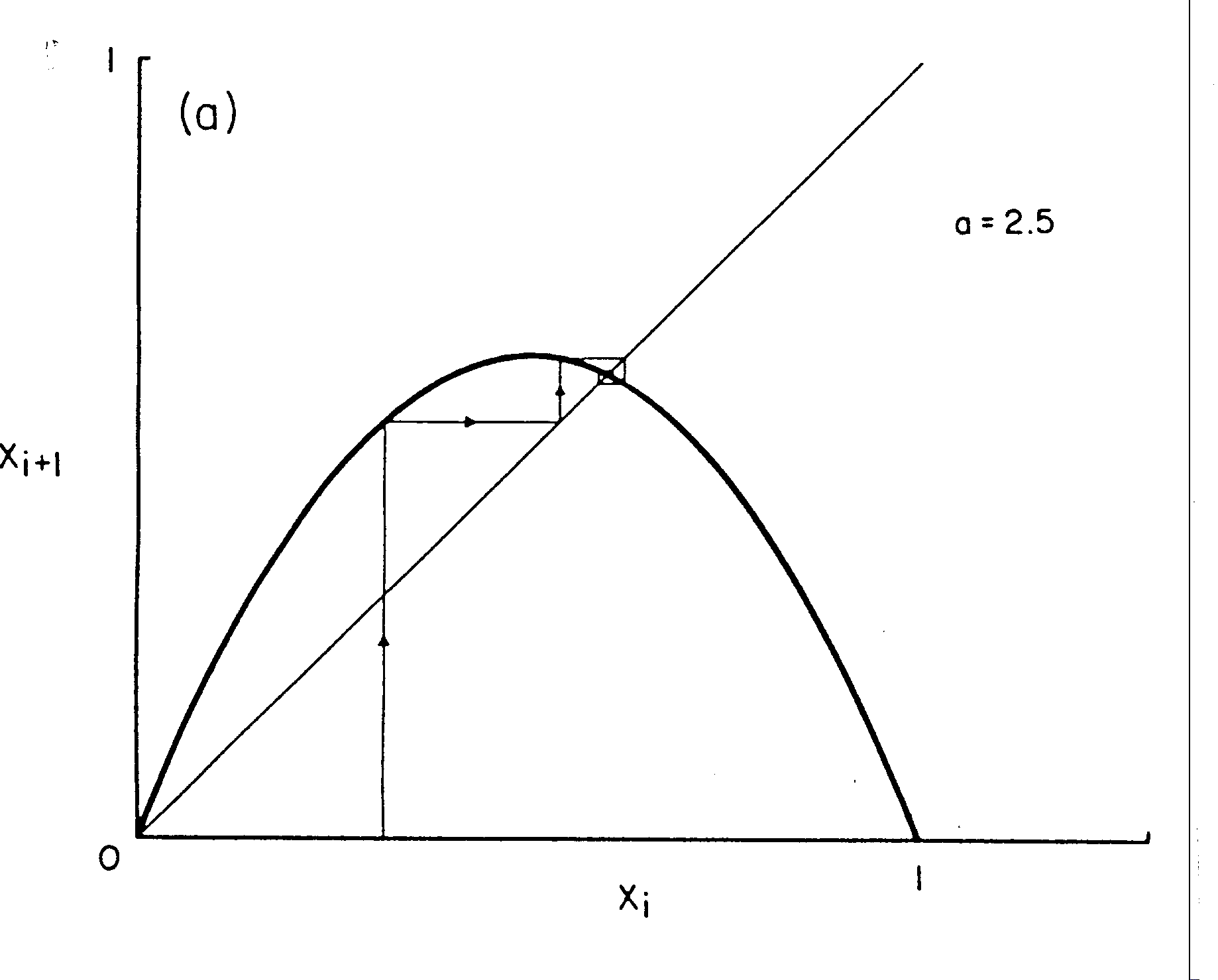
Another way to make the calculation is by a graphical method. The figure below illustrates this method.

Figure 1: The "phase portrait" for the logistic equation in the stationary realm.

The equation, which describes a parabola, is plotted in figure 1 with the particular value for A being set at 2.5. This determines the exact shape of the parabola, which is of crucial importance. The line at 45 degrees is the locus of all points for which X_n+1 = X_n. By starting with the initial value on the horizontal axis (vertical line with arrow), the new value is found by drawing a verticle line to the parabola. [On your calculator this is equivalent to multiplying the initial value of X_n by (1 - X_n )A]. Project the point of intersection horizontally to the vertical axis to determine X_n+1. Then, to do the next iteration, extend this horizontal line until it intersects the 45^o line. This converts X_n+1 into X_n for the next iteration. For this value of A (2.5), the process quickly converges on a particular stationary vale of X as can be seen on the graph as a set of ever diminishing partial rectangles. This final point represents the equilibrium for the system. [On your calculator, this value will always result in itself being calculated for X_n+1 when it is fed in as X_n.]     

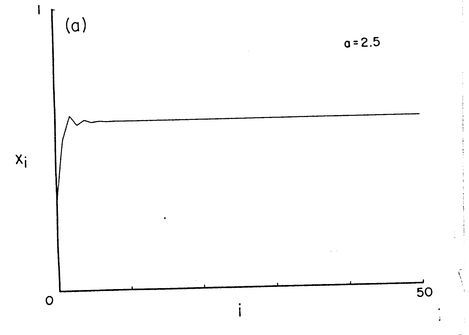
_{The next example is for a slightly higher value of A and it results in periodic behavior.}