As we explore these topics always think on how you can improve image quality and eliminate factors that reduce the quality

1. Components of an image
   1. Why do gamma cameras have "poor" resolution? Is it just the gamma camera?
   2. Background
      1. Consider the type of radiopharmaceutical being injected and to what percentage does the radiotracer go the area/organ of interest? That which does not go to the target area may translate into background (Bkg_. Can you think of examples?
         1. What about the Bkg that surrounds the area of interest?
            1. Generally, it is not specific and it may reside in bodily fluids or surrounding soft tissue. Poor collimation, septal penetration, and/or scatter my further contribute to poor image quality
            2. Extending the time between injection and acquisition and/or shifting the photopeak slightly may improve image quality
   3. Scatter (facts we already know)
      1. Cross talk occurs where gammas rays penetrate septa and are still detected outside the correct area of interest. See collimator
      2. Distance between object under acquisition and the detector causes increased scatter as the distance increases away from the source
      3. Scatter occurs when Compton interaction changes the angle of the initial gamma ray that reduces its energy, interacts with the crystal and generates a pulse height that falls within the range of the energy window and it becomes part of the image (PF)
      4. From "c" if the incoming gamma that is detected fall below then LLD is not detected (GF), but it will still be displayed on the spectrum of the energy pulses. Where would you expect to find it?
   4. Attenuation
      1. Low energy gammas attenuate via Photoelectric effect in the body habitus. But as the E_γ increases then Compton interaction comes into play. Further increases in higher E_γ will results in Pair Production. Evaluation of the chart below reveals how E_γ interact in water and what happens to the attenuating photons as its energy increases
      
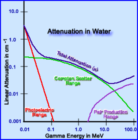
      2. In yet another application, if water is replaced with lead septa for the purpose of collimation then attenuation of gamma energy occurs in a similar fashion, however, with lead the attenuation coefficient is much greater. Why?

      
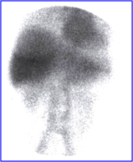
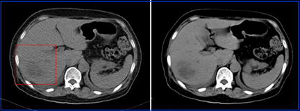
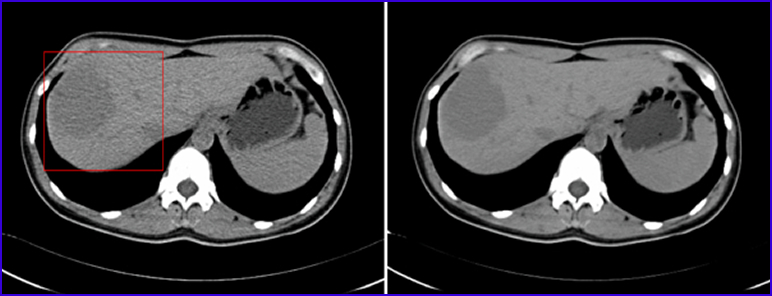
      1. This is an example of breast attenuation in an RBC scan.
   5. Noise
      1. The fewer the counts in an image (consider count density in each pixel) the more statistical variation in an image. Remember the relationship between counts and % standard deviation
      2. Low counts translates to a grainy image with poor resolution. The term used for this is noise

      
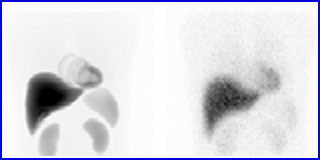
      An IAEA article - click image to go to it

      3. The image on the left has greater counts, while the image on the right has reduced counts. Attenuation and scatter may also be at play
      4. What can be done to reduce noise?
         1. Increase the amount of mCi injected
         2. Adjust your Matrix size downward - consider the resolution you need
         3. Image filtering can also reduce noise - can you think of an example? Remember this?
         
         4. Modify your collimation - apply the concepts
            1. Distance between patient and detector
            2. Scatter counts increases with distance
         5. Acquisition time/image - increase time increases counts but remember as the time lengthens patient movement must be considered
         6. Question? When is resolution not considered an important factor in image quality? Examples?

         
         http://iopscience.iop.org/article/10.1088/0031-9155/58/16/5803

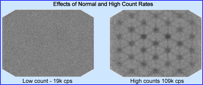
         7. Quantum mottle is a term used in CT, however it relates to NMT - A large patient has greater attenuation causing a greater loss of x-rays. The result of this is a grainy CT images because fewer x-rays have been detected. See and compare the two images above (click the image to enlarge)
         
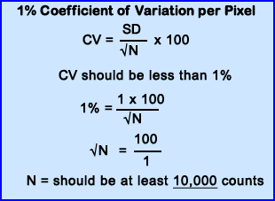
         8. Food for thought - An unattainable standard! How many counts are needed per pixel for each pixel in a 256 x 256 matrix to have 10,000 counts? Answer
   6. Two-D verses 3-D imaging
   
   1. In planar 2-D images superimposition of radioactive uptake occurs which might block the area of interest. It could completely hide the disease or blend in with another object, especially if both have similar contrast or count density
   2. This is one of the rationales for acquiring multiple angles when when acquiring planar data in same region of interest
   3. Does SPECT eliminates this problem? SPECT vs Planar - Link
   7. Patient motion
      1. This can cause image "blurring"
      2. To prevent or reduce patient movement
         1. Explain the procedure to the patient and why he/she should not move
         2. Reduce the acquisition time - whenever possible
         3. Note that SPECT is even more sensitive to patient movement! When compared to planar
2. Contrast
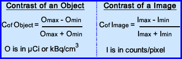
   1. Contrast is considered the ability to distinguish between different levels of radiotracer uptake within the volume being imaged. Usually the object(s) that display the contrast are recorded in counts per pixel and may be quantified in μCi/cm³. The variation of contrast and our ability to detect it is noted the formula
   
   2. When we think of what that acquired image there are several aspects that should be considered
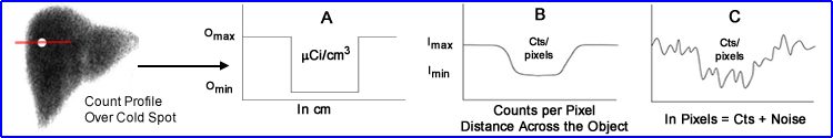
   1. In the above image a count profile is drawn over a cold spot in a liver. Now let us consider several aspects of the graph displaying the changes in image contrast
   2. The radiopharmaceutical uptake in the patient, displayed above in μCi/cm³ (A)
   3. The amount of counts per pixel show the relationship of the count distribution in the profile (B)
   4. The more realistic count distribution is one that also displays noise (demonstrates the count variation per pixel) [C]
   5. What can be done to make graph C look more like graft B?
   3. Further comments on this concept
      1. Contrast of an object occurs when the area of interest contains different levels of the radiotracer uptake. This concentration of of activity can be expressed in μCi or kBq. If the differences between these objects are slight then contrast is poor making it difficult to visualize. (because there isn't enough of a variation in the gray-scale)
      2. In nuclear medicine, we evaluate the contrast of the image by the amount of counts per pixel. The greater the variation in counts the better the contrast (%SD may also play a role)
      3. One must also consider that noise may play a rather important factor because a low count image will have a lot of noise which also effects image quality
      4. Rose criterion states that count differences between two areas must be at least 3x the statistical noises in order for a visual change
      5. Applying Contrast to Noise Ratio (CNR) and the Rose criterion the following analysis can be noted
      
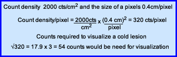
      1. Consider the above equation - If you have a count density in an area is 2000 cm² and the pixel within the matrix 0.4 cm/pixel. How many counts within this region would be needed to detect a cold lesion?
         1. Take 2000 counts and multiple by 0.4² = 320 counts are contained in each pixel
         2. The standard deviation of 320 ~17.9 counts
         3. Now multiple by three (Rose Criterion) ~ 54 counts
         4. Subtract 54 counts into 320 = 266 counts. Therefore, in order to see a change in contrast with a 320 count pixel, there must be a drop at least 266
   4. As stated above image contrast has many variables "at play" - superimposition, scatter, background, noise, and patent motion
3. In order to assure image quality evaluation of a scintillation camera is imperative! Let's take an in-depth look at these factors.
   1. System Uniformity - is the ability of an imaging system to reproduce a uniform display based on the acquisition of a uniform source of radioactivity (ie. using a uniformity flood or point source)
      1. Extrinsic uniformity can be tested by placing a collimator over on the detector then using a uniform source of activity (sheet) as the acquisition source
      2. Intrinsic uniformity is applied when the collimator is removed and a point source is placed a distance of 5X the size of the detector (FOV)
      3. Non uniformity can be seen if there is at least a 5% variation in a PMTs. To evaluate non uniformity at <5% computer analysis is required
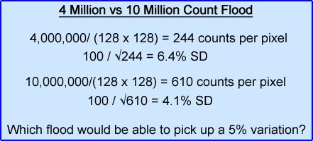
      4. While most department usually acquire a daily flood between 4 - 5,000k counts (sometimes less). Is this enough? What would be the difference between acquiring a 4,000k flood vs. a 10,000k flood?
      
      5. Non-uniformity can be due to many different factors - bent septa on a collimation, PMT failure, NaI(Tl)crystal, electronics, too much variation between the uniformity correction matrix and the acquired data
   2. Sensitivity and count rate - is the camera's ability to efficiently count as many incoming photons as possible
      1. Measurement occurs in counts/minute of the amount of μCi or kBq present
      
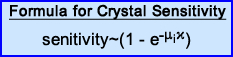
      2. Efficiency of detection is based on the formula, where:
         1. μ_i = linear attenuation coefficient of NaI(Tl)
         2. i = crystal thickness
         3. If you calculate NaI(Tl) sensitivity - calculation was done on a 3/8 inch thick NaI(Tl) crystal
         4. This application applied to the following graph
         
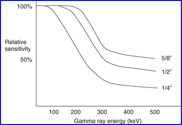
         5. As thickness increases the amount of gamma rays captured also increases as noted in the graph
         6. What should be realized is that if you increase thickness, but do not increase the gamma energy, then spatial resolution actually decrease slightly. Why?
      3. Count rates that go beyond what the system "handle" (counts/min/μCi) effects the Z pulse
         1. When the count rate gets too high two things occur: (1) pulse pile-up and (2) baseline sift
         
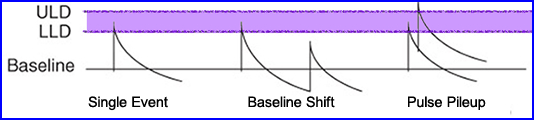
         1. Given a single gamma event noted how the energy pulse falls between the LLD and ULD. This pulse is counted
         2. If the count rate becomes excessive baseline shift can occur where the scintillating electron has yet returned to its resting state.
         3. Then a second scintillation event occurs (book - says does not return to its baseline), generating a second pulse that is lower than the first. Since the second pulse falls below the LLD, not recorded
         4. In another scenario when two Compton interactions occur next to each other that cause pulse pileup and pushes that second peak beyond the ULD
         5. Based on this situation you should be able to answer the following questions
            1. Why does the count rate drop when too much activity is present?
            2. What causes a scintillation system to drop to zero cps when the activity is exceeding hot?
            3. Why do you lose image resolution when there is too much activity?
         6. Another graph on pulse-pile up and weblink
         7. Another look at pulse-pile up effect
         2. Two methods for solving a pulse-pile up
            
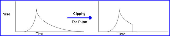
            1. Pulse clip cuts off part of the pulse by terminating its "tail" at the anode of the PMT. This allows a second pulse to be detected^-2
            2. Adjustments on clipping is a process referred to as pulse-integration time
               1. If time is set to 0.4 μsecond, the pulse is clipped and a second gamma event can be detected sooner. In this situation the amount of scintillation being detect is 81%
               2. If the clipping is adjusted to 1.0 μseconds then approximate 98% of incoming scintillation
               3. Problem - this remedy is the reduction in resolution, however, extending the μsecond does increases the amount of recording gammas
               4. What is not clear is how much activity is present in the above statements (see pp. 100-101)
         3. Second method on solving pulse-pileup and baseline shift
            
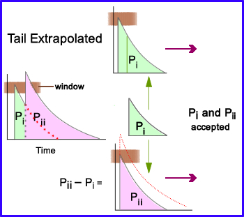
            1. Pulse-pileup has occurred as represented by the two peaks labeled P_i and P_ii with the % window (brown bar) only picks up the first peak.
            2. Pulse-tail extrapolation separates the peaks and then extrapolates the tail of the curve to P_i
            3. It then subtracts P_i into P_ii which brings Pii down to a similar size of P_i
            4. Now both peaks can be recorded within the % window
         4. It must be stated that excessive count rate: decrease system sensitivity, cause a loss in system uniformity/spatial resolution, and adversely effect energy resolution

         
         http://www.aapm.org/meetings/amos2/pdf/42-11975-5171-379.pdf

         5. Here is an example of what too much activity looks like in a flood
4. Spatial Resolution - in simple terms it is defined as an imaging system's ability to reproduce detailed information with radioactivity that has non uniform distribution (can you give an example?)
   1. Look at the basics - what effects system resolution?
      1. Intrinsic/extrinsic resolution is effected by
      2. Statistical variation in the scintillations being detected that relates to
         1. Variation in detector efficiency
         2. Mis-positioning of the scintillation events by PMT causes non-uniformity
         3. Crystal thickness
            1. Increasing crystal thickness will improve its ability to capture an incoming gamma
            2. Higher energy gammas and greater thickness further improves the crystal's efficiently

      
      4. However, increased thickness may also reduces the PMT to accurately position the scintillation event as noted in the above images (scintillating events have to travel further before being detected)

      
      http://www.aapm.org/meetings/amos2/pdf/42-11975-5171-379.pdf

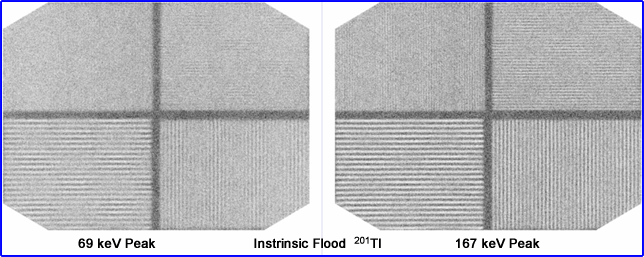
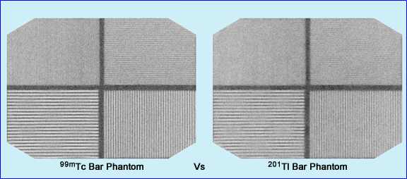
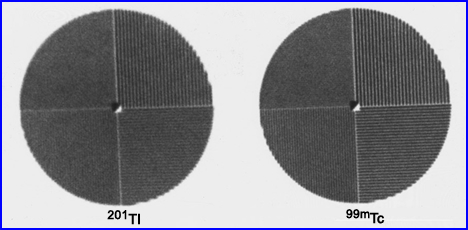
      5. Compare energy gammas and resolution based on acquiring ²⁰¹Tl at a 69 keV peak to its 167 keV peak. In nuclear cardiology, why don't we just image at the higher peak since it gives us better resolution?

      
      http://www.aapm.org/meetings/amos2/pdf/42-11975-5171-379.pdf

      6. Here is a comparison between ^99mTc and ²⁰¹ Tl bar phantoms. Which one has the better resolution. If you need a closer look, click the image

      
      http://www.aapm.org/meetings/amos2/pdf/42-11975-5171-379.pdf

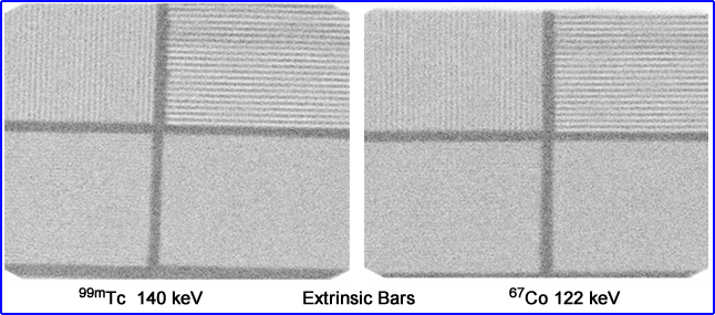
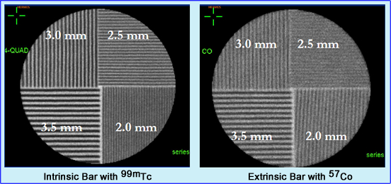
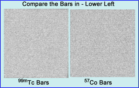
      7. A question that I have always had - What is the difference between an ⁶⁷Co flood and a ^99mTc flood? Is the resolution better in one vs. the other? Is/are there any possible implication using a uniformity correction matrix with ⁶⁷Co vs. ^99mTc? Hint - Click the image to see magnification of the 3^rd quadrant. Which shows more bars or is it too close to call
   2. Evaluating system resolution
      1. Should be done with the collimator on, a bar phantom placed below the source, a scatter medium between the detector and its radioactive source, at a distance of 10cm. Why the scatter medium?
         

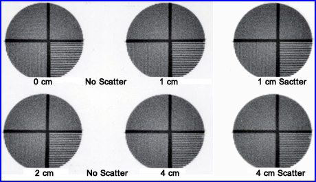
      2. The above is an example of how distance and scatter effect image resolution. As distance increases resolution decreases, but with the addition of a scatter medium resolution is further degraded
         

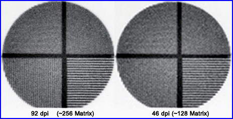
      3. Furthermore, acquisition in the wrong matrix size will cause a loss in resolution as seen above. This example shows what happens when you reduce your matrix size by 1/2. In digital imaging above its reference is in dots per inch (dpi). In nuclear medicine we prefer the term matrix size
   3. Bar Phantom
      1. The bar phantom is typically used to measure system resolution on a weekly bases
      
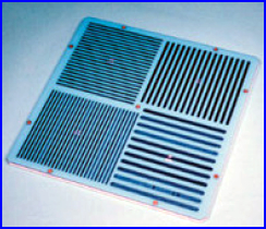
      2. It usually contains 4 quadrants of decreasing size. This type of phantom is called parallel-line equal-spacing (PLES)
      3. Standard high resolution phantom will have the following sizes (lead strips separated by plastic): 3.5 mm, 3.0 mm, 2.5 mm and 2.0 mm)
      4. These phantoms test for resolution and linearity of an scintillation camera
      5. Example of other types of phantoms
      
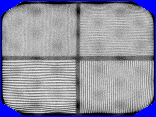
      6. The above example is a loss of linearity, were wavy lines are produced by PMT failure1

      
      Permission by JR Halama
      http://apps.snm.org/docs/CME/PresenterItems/EventID_41/PresenterItemTypeID_1/QC%20Protocols%20for%20Single%20Photon-%20Halama.pdf

      7. Which acquisition type would shows the best resolution: intrinsic or extrinsic? Why?
   4. Line-Spread Function (LSF)
      1. This gives us a more precise measurement in spatial resolution
      2. Apply an intrinsic phantom with 1 mm slits and a point source
      
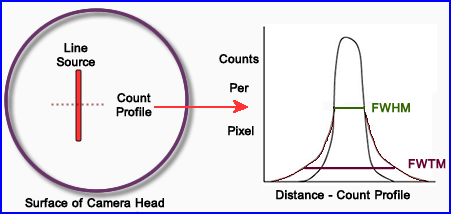
      3. More routinely the extrinsic approach is employed with the diagram above
         1. A thin capillary tube usually filled with ^99mTc is place on the surface of detector and imaged
         2. The image is then displayed and a perpendicular count profile is drawn across the capillary tube filled with activity
         3. The graphic display is usually measured in mm where the camera's pixel calibration is applied
         4. FWTM (tenth max) represents scatter while FWHM looks at system resolution
         5. FWTM also measures septal penetration in the collimator. Take this number and divide the FWHM. If the ratio is 3 times or more then there is too much scatter and a higher energy collimator should be employed
         6. If you multiply FWTH x 3 = to FWHM,where does the scatter come from?
      4. From the peak drawn above let us assume that a count profile is generated below. Calculate FWHM: If the camera's pixel size is 1.4 mm/pixel, what is its FWHM and FWTM in mm? You need to determine
      1. Peak counts = 550 counts/pixel
      2. 1/2 Peak counts = 275 counts/pixel
      3. 1/10 peak Peak = 55 counts/pixel
      4. Now determine FWHM and FWTM
      
      Count Profile of the Line Source

      Pixel #	516	515	514	513	512	511	510	509	508	507	506	505	505
      Counts	10	52	125	278	349	496	550	468	364	288	139	57	18

      
      
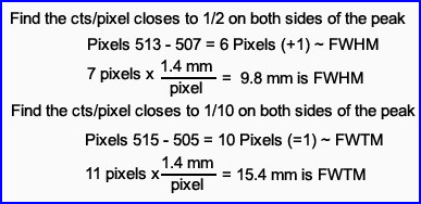
      5. What is the FWHM and FWTM values? Is there too much scatter or should the collimator require thicker septa?
      5. A second approach to evaluate the system's resolution is to place two 2 line sources at a certain distance from each other, acquire the data, move the 2 sources closer, acquire data again, and repeat until the two line sources appear as one on the acquisition

         

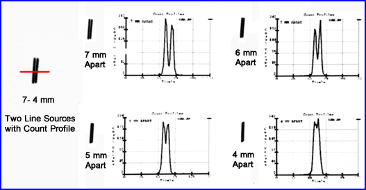
         1. From the acquired information, count profiles are drawn through each set of line sources. The data is then graphically displayed
         2. Note the results - What are your comments?
         3. From qualitative and quantitative standpoints, when do the two become one?
         4. If two hot spots are 4 mm apart, using the same resolution in the above graph, would you be able to see to distinct spots?
   5. Modulation Transfer Function (MTF) - It all comes down to this (FYI - This becomes more important when we explore the concepts of SPECT)
      1. MTF adds to the quantification process by measuring a camera's ability to identify objects of different sizes and its surrounding contrast
      2. To better understand MTF the concept of frequency domain must now be introduced
      
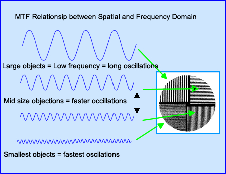
      1. The image is displayed in the spatial domain
      2. It is then converted into a frequency domain via a process known as Fourier Transformation
      3. These oscillations vary pending the size of the object being acquired. Lower frequencies contain large objects with slower oscillations while smaller objects contain faster oscillations
      4. Above the bar phantom generated four types of oscillations, can you explain why?
      
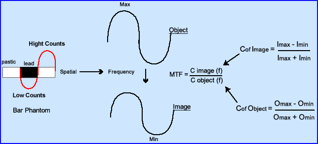
      5. This diagram further explains the relationship between spatial and frequency domains noting the relationship between image and its contrast
         1. Contrast from an image converts to its frequency
         2. Contrast of the object converts to its frequency
         3. Based on how well the system can reproduced the object a value of 1.0 to 0 is given, where 1.0 resolves the object 100% with no distortion
         4. A value of 0 resolves nothing

      

       

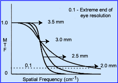
      3. From the MTF formula one could theoretically come up with different MTF values based on the evaluation of different imaging systems. Look at the above image and answer the following?
         1. Which curve has the best resolution?
         2. When is the object no longer resolvable?
         3. Which curve demonstrates the "best" blend of resolution between the different objects (small, medium, and large)?
         4. Where do you think noise and background fall on this curve?
      
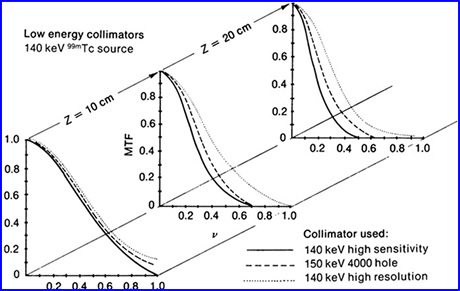
      4. A practice application to MTF can be used when comparing different collimators with response to distance from an object
         1. The 3 MTFs are located at surface, 10 cm, and 20 cm from a source of activity
         2. How do the different collimators respond?
         3. What happens as you increase distance from the source?
         4. At 20 cm which collimator has the best MTF? Resolution?
         5. What happens to the slope as you increase the distance?
         6. Notice the difference between sensitivity and resolution
      5. If you were to to consider a room full of difference sounds and then apply the concept of imaging contrast, how would they relate?
         1. Listen and think of (1) All the noise and (2) Spatial resolution
         2. Consider noise
         3. Size of an object vs what sounds can you hear
   6. Bar Phantoms (BP), LSF, and MTF
      1. BP and LSF
         1. Look for where the camera resolve the smallest bars and this is where you'd apply FWHM concept
         2. Take the value of any FWHM and divide by 1.75 to get your spatial resolution
         3. Example - If FWHM = 9 mm/ 1.75 = 5.1 mm
         4. Based on this value the smallest object your imaging system will be able to resolve down to 5.1mm
         5. Does this fit into our definition that states, you need to have 3 pixels cover an object in order to resolve it?
      2. BP and MTF
         1. Refer to the MTF curves above and note that there are four frequencies being generated
         2. This controlled situations allows for better assessment of the imaging system
         3. How well do you think you can resolve the bars at 2.0 mm based on the image above? (it's the smallest bars)
      3. MTF and LSF blends the concepts of contrast and resolution
5. Acquisition parameters - there are 4 considerations
   1. Counts/time
      1. Getting enough counts (as a general rule) is not usually as big a deal in planar imaging as compared to SPECT
      2. What occurs when you get enough counts?
         1. Increased counts reduces statistical variation, but what happens when you apply acquisition time?
         2. Does increasing the imaging time increase the probability of patient motion?
         3. On the other side of the concept if you are attempting to acquire a dynamic process, how is temporal resolution applied?
      3. Choice of Collimator
         1. Always consider using the right collimator base on the energy photon being acquired
            
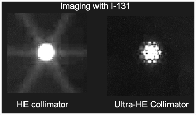
            Obtained from SNM, 2000 by Dearaja YK et. al.
            1. The above example shows the difference between imaging a point source with a HE collimator vs. one that is "ultra" HE collimator (collimator designed for 511keV gamma). What do you think caused the elimination of the star defect?
            2. Always employ the right collimation that is based on the energy gamma. As a rule of
               1. Up to 200 keV - LE
               2. 200 - 300 keV - ME
               3. Greater than 300 keV - HE
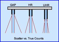
            3. Consider your choices regarding a GAP and UHR and the need to acquire a high count image. What are the advantages/disadvantages of each?
            4. If you are interested in acquiring a lot of counts in a region, but do not care about resolution, what type of collimation would you choose?
   2. Image matrix
      1. Match up the right size based on the amount of count that you need to acquire
         1. Consider the differences between 64 - 128 - 256 matrix
         2. If you need high resolution and you acquire in a 64 x 64 matrix, are you get great resolution?
         3. If you initially acquired an image for 1 minute at a 128 matrix and got 250k counts, what would happen if you required another 1 minute image in a 256 matrix?
   3. Energy window
      1. Consider your LLD and ULD settings ...
      2. If you normally acquire most of your data in a 20% window ... What would happen if you changed to departmental protocol where a 30% window? Or if you changed it to a 15% window?
      3. What happens when you shift the energy window slightly to your right when acquiring data?
      4. Note the angle of scatter
         1. A 140 keV gamma with a 10% window will have gamma ray scatters of up to 50^o
         2. An 80 keV gamma with a 10% window will have a scatter angle of 73^o
         3. Hence the lower the energy the more Compton scatter enters your window
   4. Object-Collimator distance
      1. Increasing distance between these two does what to resolution?
      2. Decreasing distance between these two does what to resolution?

Quality Assurance Testing of Gamma Camera and SPECT Systems by SL White, UAB (2010). Attained from AAPM annual meeting.

2-Physics in Nuclear Medicine S.R. Cherry p.233

3 - Image Quality in Nuclear Medicine (slice 24) [http://www.slideshare.net/jdtomines/image-quality-in-nuclear-medicine]

Much of the lecture material in the section was attained from Chapter 8, Image Characteristics and Performance Measures in Planar Imaging. Nuclear Medicine Instrumentation by J. Prekeges

Objectives

1. When considering imaging quality think: background, scatter, attenuation, noise, difference between 2D and 3D, patient motion.
2. Compare contrast to counts.
3. Apply the rose criterion.&
4. Consider system uniformity with the amount of counts in an AM flood.
5. Apply the concept of pulse pileup to baseline shift and pulse clipping.
6. Assess system resolution intrinsically and extrinsically.
7. Calculate FWHM and FWTM.
8. Define MTF and the location of: large objects, small objects, background, and noise.
9. Determine the type of collimation used based on the energy gamma.