- Most imaging systems have analog-to-digital converters (ADC) which takes the data acquired from the PMT and then digitizes the the information into a matrix with X and Y coordinates
- The more pixels you have in an image the greater the resolution
- In nuclear medicine a key factor to better resolution is associated with the amount of pixels in an image
- The matrix size defines the amount of pixels in an image. To simplify this discussion let's look at a 3 x 3 matrix that contains 9 pixels
- The above matrix shows a count value in each cell notices that it decreases in descending order with the lower right containing 50 counts and upper left at 0 counts.
- This variation in counts shows a variation in the gray scale where increasing shades of gray relates to a decease in the number of counts
- A gray scale has 256 shades (28) of gray that relates to the amount of counts in an image
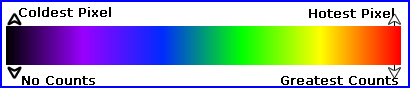
- When displaying counts from an acquisition the computer applies a Look-Up Table (LUT) that assigns counts/pixel with XY coordinates
- Given the above gray scale the pixel(s) with the maximum number of counts is white (or clear) and the pixels with the least counts is black
- A gray scale can also be inverted where the hottest pixel becomes black and white indicates no counts. This is referred to as inverse video
- LUT can also be assigned to many types of color scales which may further enhance the imaged data and may improve the diagnostic quality of a study
- LUT combinations use up to three primary colors are Red,Green, and Blue (remember ROYGBIV?)
- A blending of colors increases the amount variation between the amount of counts to pixels and the amount of color shades per count(s)
- This further increases the ability to find minor changes in counts when all three primary colors are used. Perigees states 262,000 shades or combinations can be used, however, if each color represents 28 shades then there are 28 x 28 x 28 = 1.67 x 10⁷ (red, green, and blue) combinations
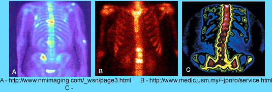
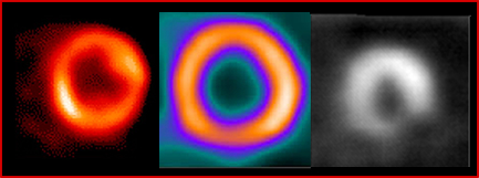
- Example of how different color scales effect how we visually see a bone scan
- What kind of detail can we actually see?
- Related to shades of gray the human eye can only see about a 2% change in brightness. Therefore, given 256 shades of gray, it takes 5 shades in either direction to realize a slight change in the scale
- The human eye can see over 1 million types of color, hence the eye is more "sensitive" to a tricolor scale
- Yet the human eye is more sensitive to green and yellow when compared to blue and red
- Understanding our Sluts and NM "limited" resolution it can be stated that minor changes in counts per pixel may not be seen
- Test our ability to see minor changes in color (hue). There are 4 rows. The first and last blocks in each row cannot be moved. Arrange the boxes within the row to match the subtle changes in color. Click Test
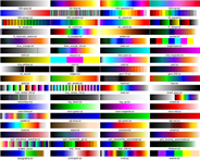
- Here are a lot of examples of LUTs used in nuclear medicine and diagnostic radiology. Click the image to enlarge
- Looking at nuclear cardiology displaying the LUTs, which scale would you choose?
0 |
5 |
15 |
20 |
25 |
30 |
40 |
45 |
50 |

- Pixel size
- Identification of pixel size is noted above with a 128 matrix and a camera that is 15 inches square
- This information is helpful, not only in assessing resolution, but also being able to measure the size a lesion - How would you measure the size of a lesion?
- Nuclear medicine matrix sizes vary and are as follows
- 32 x 32 (flow study)
- 64 x64 (flow study)
- 128 x 128 (flow or static images)
- 256 x 256 (static images)
- 512 x 512 (static images)
- 256 x 1024 (whole body scan)
- 512 x 1048 (whole body scan)
- The question one has to ask is which matrix is the best choice given a specific procedure? While examples are given above there is still some variation with certain imaging procedures
- KEY - When selecting a matrix size you need to know
- The amount of counts being acquired
- Type of collimation
- Another issue of concern is the byte verses word mode of the pixel
- A bit in computer language is has the value of a 1 or 0
- Consider 16 bit = 2 byte = 8 = 1 word. How many counts can a pixel hold?
- If a matrix size is 128 x 128 x 1 byte then it means that each pixel can hold 28 counts or up to 256 counts. How many pixels are there?
- What happens if a pixel becomes saturated or counts go beyond 256?
- The image stops acquiring (this is my personal experience) or
- The pixel stops acquiring, but the rest of the system continues to count or
- Counts in the saturated pixel roll over and start back at zero and build up again
- A pixel can also be in word mode which translates to 28 x 28 = 65.5k counts/pixel. Chances of pixel saturation is slim to none. Most modern cameras have the ability to collect in word mode
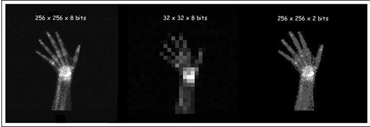
- Here is an example how how resolution is effected by matrix size and depth
- More information on bits and bytes
http://en.wikibooks.org/wiki/Basic_Physics_of_Nuclear_Medicine/Computers_in_Nuclear_Medicine
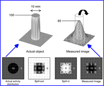
- Partial volume effect (PVE)1
- This is best explained by looking at the edge of a circle (above) where only part of a pixel is collecting the counts
- The result is a lost of counts at the edge of the image's acquisition
- In the exam given the actual image is circular, but pixels are squared
- This means that certain areas of the cylinder collects less counts based on the fact that only part of the pixel is collecting data
- Activity spills out from the cylinder into the partial pixel(s)
- Likewise activity also spills into the pixel that are outside the cylinder which is considered background
- Net result is referred to as PVE
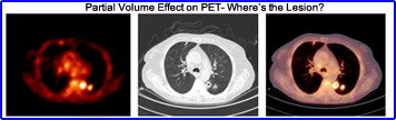
- Here is how PVE can actually confuse the acquired data. In the above image a PET scan defines a tumor that may or may not be attached to the thoracic wall. CT shows that is it not part of the wall and the fused PET/CT scan helps the physician negate the PVE effect. Another point of interest is that the matrix for the above image in PET is 128 whereas the CT image has a matrix of 512
- Does a greater amount of pixels reduce PVE?
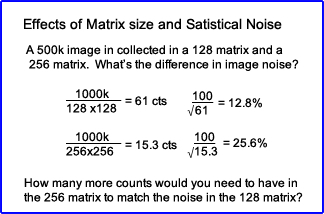
- Matrix size and statistical noise
- Assume you collected 1 million counts in a uniform flood that has a 128 matrix? What is the percent coefficient of variation?
- What happens to the CV if you collect the same amount of counts in a 256 matrix?
- How many counts to do have to attain in the 256 matrix order to have the same variation that is in the 128?
- Does too much error (noise) cause problems in our image quality?
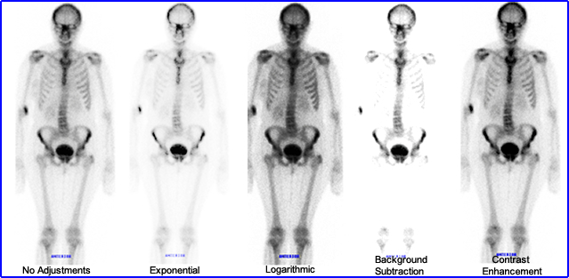
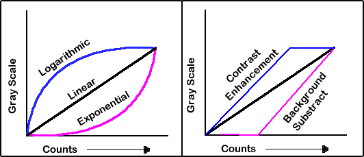
- Images can be adjusted in different formats - above is the graphical display and below is the visual results
- Raw data is displayed on a linear curve as counts increase so does the gray scale
- In a high count image a logarithmic adjustment can be made which enhances the low count pixels while the higher count pixels have less variation
- In a exponential adjustment the low count pixels have little variation, however, the higher count pixels show a greater change in gray
- Background subtraction gives ever pixel the same gray (zero) until the curve begins to rise
- Contrast enhancement gives the hottest pixel value to all pixel in the plateau where variation in gray occurs as the curve begins to drop
- Here is what different adjustments actually do to the image. The image on the far left has not been adjustment
- Images can also be adjusted with different types of filters
- Convoluted kernel (a term used when filtering an image)
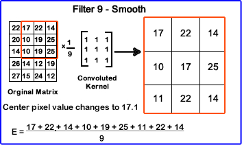
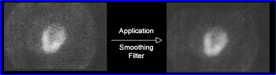
- First look at a smoothing filter
- Components - Raw data + convoluted filter = output of modified counts. Another way of stating this, raw data is manipulated by adding a mini matrix (convoluted kernel) with a numeral value that will in some form alter the original matrix
- The convoluted kernel multiplies every pixel by 1 and then divides the center pixel by 9
- This operation is done to every pixel in the original matrix (raw data)
- Above is the results of a smoothing filter
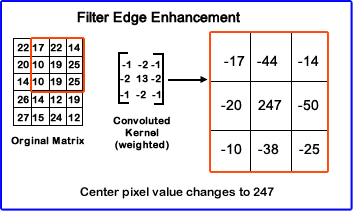
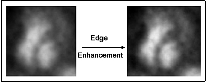
- Edge Enhancement filter (kernel)
- In a variation of filtering a weighted kernel, as seen above, has different values within its mini matrix which alters the raw data in a completely different fashion
- Notice the center pixel within the kernel is the only positive value all others are negative
- The net result causes those pixels with higher counts significantly enhanced
- Filtering had many applications in nuclear medicine as well as other areas of digital imaging. Wiki has an interesting link regarding the many types of filter applications and the convoluted kernels that go with it
http://www.slideshare.net/brucelee55/processing-methods-of-nuclear-medicine-images
- Size
- In order to determine resolution you must first identify your area of acquisition or the size of the detector head
- If the imaging area is 400 mm and you are using a 32 x 32 matrix, what is the size of each pixel?
- This can be calculated as follows 400 mm/32 pixels = 12.5mm or 1.25 cm/pixel
- This means that each pixel represents 1.25 cm in size
- If a photon deficient area is 3.0 cm in size then hypothetically you should be able to resolve it since your pixel size is smaller than the area deficient of counts
- However, if the photon deficient area was 6 mm in size then you are going to miss it because the disease process is smaller than the system resolution
- Therefore, increasing your matrix size becomes critical in resolving the smaller area (cold or hot)
- Resolution and a 64 x 64 assuming our imaging area is 400mm x 400mm
- 400mm/64 = 6.25mm/pixel
- At this point the ability to visualize that 6 mm cold spot is almost the same of a pixel
- Realistically you should applied a 128 x 128 matrix so you can further improve your resolution. Doing this gives a pixel size of 3.25mm
- Note: The same logic above can be applied if the area under question whether it is hot or cold
- Every time you increase the matrix you increase the required storage space on the hard drive. Processing time also increases by a factor of 4
- Key Point - Determine the best imaging resolution for the system
- As stated in your reading material a typical detector size might be 15” x 20” or 400 x 500 mm.
- Using a LEHR collimator that can resolve an 8 mm object at a depth of 10 cm (this means that the FWHM is 8-mm)
- Hypothetically it is suggested that you reduce the mm/pixel to the system’s resolving ability
- However, sampling resolution has determined that it takes three times that amount
- So if the FWHM is 8-mm, then the mm/pixel should be 8 mm/3 = 2.7
- If a 128 matrix is used what is the mm/pixel? 500 mm (detector)/128 (matrix) = 3.9 mm/pixel. Technically this isn't small enough
- Applying a 256 matrix is suggested 500-mm/256= 2.0-mm/pixel
- Hence, the 256 x 256 matrix is what is needed to resolve down to a 8 mm object. What is the pixel size?
- Homework assignment: Pixels and resolution - This assignment uses the above data to determine system resolution.
- Frame Mode
- Consider this a static mode where counts addressed to XY pixel coordinate within the matrix
- During acquisition the image is held in an image buffer and then stored once the acquisition is stopped, on the hard drive
- In a dynamic mode the computer usually has two image buffers where counts are acquired on the first one, then when the time per frame ends the acquired image is storage while the next image being acquired continues with buffer #2
- Matrix size is also important since larger matrix sized would take longer to store
- Therefore, dynamic images are usually acquired in a 64 matrix
- Balance the concepts - dynamic image, amount of counts, and the size of the matrix
- Gated Frame Mode
- In this case, the amount of buffers equals the number a frames being collected
- The frame state is triggered by the R wave and collected over a very short period of time
- Each R wave starts the frame state and counts are collected until a certain level is achieved
- If there is a variation in the heart rate then usually the end frame(s) will lack activity at the end of R wave causing a winking out effect
- Gated studies can be set to reject irregular beats and when this happens then the buffers return to zero counts await the next good R wave
- List Mode
- This does not place counts into a buffer but instead saves all counts with XY location and stores them individually
- Good example where is might apply is cardiac gating where every frame is individually collected
- If applied, all counts, XY locations, with every R wave is saved. Then the technologist picks which R waves are acceptable, composing the correct cardiac cycle. That is the ones that have normal contractions
- This type of acquisition is rarely used
- Digital Zoom (post vs pre)
- In this case of zooming after the image is acquired
- If you acquired in a 128 matrix and then magnified the image by x2 the result would cause you to have an image that would now be 64 pixels on the viewing scree
- This results in a loss of resolution
- Zooming prior the acquisition improves resolution
- Consider the 128 matrix being acquired has a magnification of x2. Compared to the non-zoom, the pre-zoom is imaging 1/2 the imaging area with the same amount of pixels
- Therefore, improves resolution
- In this case of zooming after the image is acquired
- There are numerous types of displays devices which you can read about in your book
- Key points to remember are
- Nuclear medicine resolution is limited
- The display device resolution should be at least as good as you imaging resolution
Return to the Beginning of the Document
Return to the Table of Content