Probability and Statistics

1. There are many factors in NMT that effect the imaging results of an acquired procedure:

Peak	Where does statistics relate to these concepts?
High Voltage
Statistical flux
Pixel size
Gray scale
Acquisition time and the amount of counts
Activity injected to patient

2. This issue is that error can occur with any of the variables stated - error might happen during acquisition and/or processing of data? As a technologist, you are responsible to minimize error as much as possible. Types of error
1. Error is a measurement where there is a difference between the true value and variation being measured
2. Blunders (error) are so obvious in nature that they are easy to detect (can be prevented)
   1. Incorrect set (wrong peak) with imaging equipment
   2. Injecting the wrong radiopharmaceutical
3. Determinate error are known systematic error, this can be caused by (usually something that is unavoidable):
1. Experimental design
2. Malfunctioning equipment
3. Lack of correction from external influences (lack of counts in an image)
4. Indeterminate error is yet another form, it is also known as random error
1. Things that cannot be reduced by correcting for those external factors
2. Radiation decay is a random event, hence it is considered a form of (indeterminate) statistical error
5. Types of error can also be defined from the diagrams below
1. Inaccurate, unbiased, and imprecise
2. Inaccurate, biased, and precise
3. Inaccurate, biased, and imprecise
4. Accurate, unbiased, and precise

5. What is the difference between precession and accuracy? Answer
3. Poisson Distribution is another term used in statistics which is applied to our science
1. When considering radioactive decay it should be noted that the number of dpm is only an average, it is not a constant
2. Disintegration of a radioactive atom is a random event and hence decay is considered a random variable
3. If you count a source for one minute and recount it the following minute its cpm will most likely be different
4. Half-life is only an average and not necessary considered a "true" value
5. This website states that ^99mTc has a T_1/2 of 6.03 hours yet this other link shows it at 6.02 hours
6. When considering precision and accuracy of a radioactive sample one must consider the randomness of decay (note: the greater the counts collected the less error is given to the analysis of the equation). Examples of where error can be an issue with a nuclear exam:
1. Number of counts being accumulated or time necessary to acquire a certain amount of counts
2. Dose to be administered to the patient (the greater the dose the more the counts)
3. Scan speed when looking at whole body imaging (the slower the scan the more counts collected)
4. Amount of counts/slice in a SPECT scan
4. Counting a sample of activity and its relationship to Poisson distribution
1. Consider counting a ¹³⁷Cs source 25 times and then graphing it below. A distribution of counts will generate a bell curve - Poisson distribution

2. Now let us considered standard deviation (SD)
3. As compared to the distribution above let us take a look at a normal SD using Poisson distribution. Note how the graph above and below are similar in design

1. From the graph above N = the number of counts collected which is 10,000 counts that shows its distribution along a bell curve.
2. One SD of 10,000 counts is 1,000 demonstrated by the smaller bell.  To determine SD you must find the square root of the total counts



3. Now let us take a look at effects on the amount of counts as it relates to the SD

4. From the above table one can consider several points
1. Increasing the number of counts decreases the percent error and reduces statistical error
2. Increasing the number of SD increases the range, increases the percent error, and improves statistical accuracy
5. Hence it is important to realize the importance of increasing counts in a sample in order to reduce the percentage of error (and %SD)
6. Another interesting point is to look at how the change in counts (increased counts effects SD and Poisson distribution
1. Less counts shows a curve with a larger width
2. Increased counts shows a curve with a decreased width
5. How many counts does one need to have enough counts where the percent error is not significant?
1. As a rule of thumb - 10,000 counts is considered adequate
2. Consider √10,000 = 100 where 1 SD = 100
3. Consider the sample error, 100/√10,000 = 1% for one SD
4. By increasing your % error you increase your level of confidence - 2 SD = +/- 200 (2%) and 3 SD = +/- 300 (3%)
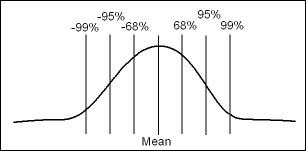
5. Further analysis of percent error can be noted from the table above
6. What about Counts and confidence intervals?
1. 1 SD = 68%, which means that in any given population 68% of the sample will fall in that range
2. 2 SD = 95%,
3. 3 SD = 99%
4. Hence the greater the number of SDs the greater the probability that your sampling will fall within that appropriate range
7. More on count sampling
1. Mean - is the value (counts) obtained by adding together all the counts from every sample collected and dividing by the total number of data sets collected
2. Median - when values (counts) are placed in order of magnitude (smallest to largest), the median is the center value, which lays half way. Also referred to as the 50^th percentile
3. Mode - is the value (counts) that appears most often in the data set
8. Applying SD where more than one sample is being counted
1. When a radioactive source is counted numerous times (at the same time interval) a number of counting samples are generated. If one were to graphically display this the distribution would appear as a bell shaped curve
2. As stated before this is how Poisson distribution fits in. This is similar to Gaussian distribution which also generate this bell shaped curve
1. Poisson distribution is used to determine the mathematical probability that an event will occur. By analyzing a series of events a mean number can be generated. By applying a SD one can then determine the statistical probability of the next event. Hence SD is used to note the amount of times an event will occur within a specific range or frequency.  Example - 2 SD takes into account that any future events will have a 95% probability that it will occur within the same range.  As you increase the amount of %SD you increase the probability catching the next occurrence.  To assess multiple events the following formula is applied:



2. Application - If you were to count ¹³⁷Cs 10 times in a well counter you would get 10 samples and the formula above is used to calculate the standard deviation from the mean
3. The table below demonstrates the actual events and calculations used to determine SD




4. If graphed, the events would be distributed accordingly along a bell shaped curve



9. Now let us look at Chi Square (X²)
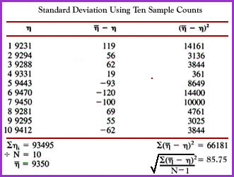
1. The actual definition is found here. In the nuclear medicine arena it is testing to see if a counter (ex. well counter) is recording counts that are "true."  You could say that you are testing a detector's reliability to correctly detect counts from a source of radiation. What we do know is that decay is random, which means that the counting instrument is counting in a random fashion. Therefore there must be enough variation in counts to pass the test.  The formula for X²



2. Now let us apply the formula where n = the number of times a ¹³⁷Cs sample was counted in a well counter. The average of those events is determined, then subtracted by each event. The events are then squared and the total value is summed. This value is then divided by the mean. Those calculations are noted below





3. Next you must apply the degrees of freedom which is determined by the following formula (N - 1) = degrees of freedom (df)
1. N = the amount of sample counts taken, usually this value is 10
2. Subtracting by 1 the degrees of freedom becomes 9
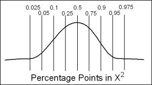
3. You then want your X² value falls between 0.1 and 0.9. Does it?
4. If it were below 0.1 what would that mean?
5. If it were above 0.9 what would that mean

df	0.995	0.99	0.975	0.95	0.90	0.10	0.05	0.025	0.01	0.005
1	---	---	0.001	0.004	0.016	2.706	3.841	5.024	6.635	7.879
2	0.010	0.020	0.051	0.103	0.211	4.605	5.991	7.378	9.210	10.597
3	0.072	0.115	0.216	0.352	0.584	6.251	7.815	9.348	11.345	12.838
4	0.207	0.297	0.484	0.711	1.064	7.779	9.488	11.143	13.277	14.860
5	0.412	0.554	0.831	1.145	1.610	9.236	11.070	12.833	15.086	16.750
6	0.676	0.872	1.237	1.635	2.204	10.645	12.592	14.449	16.812	18.548
7	0.989	1.239	1.690	2.167	2.833	12.017	14.067	16.013	18.475	20.278
8	1.344	1.646	2.180	2.733	3.490	13.362	15.507	17.535	20.090	21.955
9	1.735	2.088	2.700	3.325	4.168	14.684	16.919	19.023	21.666	23.589
10	2.156	2.558	3.247	3.940	4.865	15.987	18.307	20.483	23.209	25.188
11	2.603	3.053	3.816	4.575	5.578	17.275	19.675	21.920	24.725	26.757
12	3.074	3.571	4.404	5.226	6.304	18.549	21.026	23.337	26.217	28.300
13	3.565	4.107	5.009	5.892	7.042	19.812	22.362	24.736	27.688	29.819
14	4.075	4.660	5.629	6.571	7.790	21.064	23.685	26.119	29.141	31.319
15	4.601	5.229	6.262	7.261	8.547	22.307	24.996	27.488	30.578	32.801
16	5.142	5.812	6.908	7.962	9.312	23.542	26.296	28.845	32.000	34.267
17	5.697	6.408	7.564	8.672	10.085	24.769	27.587	30.191	33.409	35.718
18	6.265	7.015	8.231	9.390	10.865	25.989	28.869	31.526	34.805	37.156
19	6.844	7.633	8.907	10.117	11.651	27.204	30.144	32.852	36.191	38.582
20	7.434	8.260	9.591	10.851	12.443	28.412	31.410	34.170	37.566	39.997
21	8.034	8.897	10.283	11.591	13.240	29.615	32.671	35.479	38.932	41.401
22	8.643	9.542	10.982	12.338	14.041	30.813	33.924	36.781	40.289	42.796
23	9.260	10.196	11.689	13.091	14.848	32.007	35.172	38.076	41.638	44.181
24	9.886	10.856	12.401	13.848	15.659	33.196	36.415	39.364	42.980	45.559
25	10.520	11.524	13.120	14.611	16.473	34.382	37.652	40.646	44.314	46.928
26	11.160	12.198	13.844	15.379	17.292	35.563	38.885	41.923	45.642	48.290
27	11.808	12.879	14.573	16.151	18.114	36.741	40.113	43.195	46.963	49.645
28	12.461	13.565	15.308	16.928	18.939	37.916	41.337	44.461	48.278	50.993
29	13.121	14.256	16.047	17.708	19.768	39.087	42.557	45.722	49.588	52.336
30	13.787	14.953	16.791	18.493	20.599	40.256	43.773	46.979	50.892	53.672
40	20.707	22.164	24.433	26.509	29.051	51.805	55.758	59.342	63.691	66.766
50	27.991	29.707	32.357	34.764	37.689	63.167	67.505	71.420	76.154	79.490
60	35.534	37.485	40.482	43.188	46.459	74.397	79.082	83.298	88.379	91.952
70	43.275	45.442	48.758	51.739	55.329	85.527	90.531	95.023	100.425	104.215
80	51.172	53.540	57.153	60.391	64.278	96.578	101.879	106.629	112.329	116.321
90	59.196	61.754	65.647	69.126	73.291	107.565	113.145	118.136	124.116	128.299
100	67.328	70.065	74.222	77.929	82.358	118.498	124.342	129.561	135.807	140.169

6. What do we use those values?
1. The value fell below 0.1 then the likelihood of that event falls way below left tail of distribution
2. If the value fell above 0.9 then the likelihood of that event falls way above the right tail of distribution
3. Less than 0.1 means there is not enough variation
4. Greater than 0.9 means there is too much variation
5. Note the distribution of this frequency in the graph below