Note: From your renal quantification lecture we have discussed the ideal way of acquiring and processing a renography, however, the samples given below are examples of how renography is applied at certain clinics in the Louisville area. Note the differences and similarities from your renal quantification lectures.
- The first example is that of a normal renal scan
- All acquired images from the study are displayed along with the process data
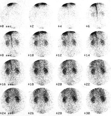
- Two second flow study is the initial analysis of the bolus injection (left image)
- From a qualitative standpoint look at the 2 second flow study and notice that as the activity goes down the descending aorta both the left and right kidneys "light up" at the same time. This is an indication of normal uptake
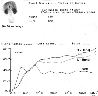
- Quantitatively regions of interest are drawn around the left/right kidney and third region is drawn around the upper portion of the descending aorta
- Time activity curves are displayed showing uptake of the both kidneys by the rise of both curves
- The curve that displays the descending aorta shows initially a rise and then a drop as the bolus passes through
- Quantitatively the Perfusion Index is calculated by taking the peak activity from the descending aorta dividing it by the activity in the left or right kidneys times 100
- Normal value is anything less than 150
- Values are within normal limits in this study
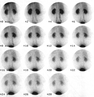
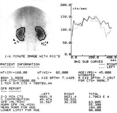
- The second set of images area displayed in summed two minute intervals, up to 30 minutes
- Qualitatively images show a continued increase of activity up to or between the 4 to 6 minute image
- Activity is then seen leaving the renal pelvis and then dumping into the urinary bladder
- Also note how background activity disappears in the upper portion of the first set of images - liver and spleen/vascular structures
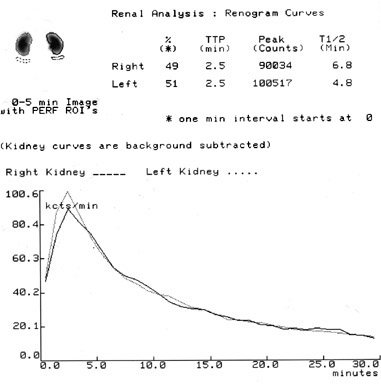
- Quantitatively (right)
- Regions are drawn on a 0 to 5 minute summed image
- Split renal function is 49 and 51 percent
- Maximum count image at 2.5 minutes (both)
- Both T1/2 are less than 10 minutes
- The second is an example of an abnormal scan
- There is no qualitative data available, only quantitative
- Image to the left shows the first 400 seconds of acquired data which was probably collected over 30 seconds per frame
- Regions of interest are drawn with appropriate backgrounds, however, it should be noted that the descending aorta was not used
- Syringe counting was used
- Other data was also entered, which includes: age, weight, height, hydration, etc.
- Notice that the normal GFR rate is below the actual data collected
- Time/activity curve is abnormal
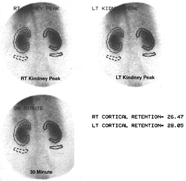
- On the second set of images (right) it shows where the ROIs were drawn
- Data calculates cortical retention
- Cortical retention should be less than 20%
Return to the beginning of the document
Return to the Table of Contents