- Determining the matrix size
- For a SPECT procedure the field of view (FOV) of a digitized gamma camera will have either a matrix size of 64 x64 or 128 x 128
- Based on sampling theory a pix le size should be 1/3 of the camera's FWHM. Additionally,
when considering the quality of image resolution factors that affect are:
- The value being measurement must be done at the center of its rotation (the farthest point from the imaging area)
- Type of collimation
- Distance from the patient
- Application of zooming - doing so will improve image quality
- Determination the right pixel
size for SPECT imaging
- When considering matrix size and resolution you must first look at the camera's FWHM. For the best possible resolution the pixel size should be about 1/3 its value.
- Therefore, if a camera's FWHM is 21 mm then the pixel size should no larger 7 mm (For more information look at this lecture as it applies to planar imaging)
- So how do you apply this data to a specific camera?
- Apply the above formula with the following data: camera's FOV = 475 mm , matrix size is 64 x 64 matrix, and no zoom is applied. The result is approximately 7.4 mm per pixel. Therefore, because 7.4 is close to 1/3 of the camera's FWHM, then a 64 matrix should be used in SPECT
- If you zoom the image by 1.5 then the pixel size drops to 4.7 mm
- If you decide to image with a 128 matrix that doesn't have a zoom the pixel size is drops to 3.7 mm
- Comment: Most SPECT acquisition only require a 64 x 64 matrix because the pixel size in mm is usually <1/3 of the FWHM

FOV = Widest portion of the imaging field Z = Zoom factor N = Number of pixels (64 or 128) D = Size of pixel - Now we need to consider the signal-to-noise ratio
and associate this with matrix size
- Generally the more noise you have the poorer the imaging quality. SPECT images usually have fewer counts when compared to planar, therefore SPECT images will contain more noise.
- Assume you collect two sets of images (64 and 128), both containing the same amount of total counts
- The 3-D matrix contains 3.84 x 10⁶ counts
- The question is how does noise effect image quality in these two matrix sizes.
- To determine the amount of noise in each matrix the equation above must be applied
- Compare the increase of noise, between a 64 and 128 matrix
- Crunching the numbers shows us that % noise increases by a factor of 2.8 when we increase the matrix size. The result is additional high frequency noise in the 128 matrix. Why does this happen? Consider a 128 matrix has 4x the amount of pixels means there are is a lot more space for a limited amount of counts
- How much longer must you acquire data in a 128 matrix to have the same SNR is in a 64 by 64 matrix? That issue is solved below
- Step 1 - Determines the amount of counts needed for a 128 image by finding the amount of counts in X. The total amount of counts required, to have similar SNR is 3.447 x 10⁷ counts in the 128 matrix
- Step 2 - Identifies the amount of cps in the 64 x 64 matrix. The amount of counts per slice is assumed to be 25 seconds/slice . Decay is not being considered. Counts per second = 2400
- Step 3 - Determines total time required to collect 3.47 x 10⁷ counts at a count rate of 2400 cps. It will also be assumed that there are a total of 128 slices being acquired at 1/2 time per slice (12.5 second/slice) when compared to the 64 matrix. Total time is approximately 241 minutes
- Step 4 - Defines the amount of time required to collect 3.84 x 10⁶ count in the 64 x 64 matrix. Time required is 26.7 minutes
- Hence, in order to collect a the same SNR value in the 128 we could have collect an additional 214 minutes. Obviously, these numbers far exceed the any expectation that a patient could tolerate

V # of voxels in circular FOV N Total counts in 3-D image % Noise Noise generated

- Ideally a filter's role is to enhances image quality, without significantly altering the raw components of the input data
- Incorrect filtering, over, or under can do any or all of the following to our image quality: reduces resolution, effect contrast, increase noise (high frequency), increase background counts (low frequency), can blur detailed information, and/or make the image too grainy
- Correct filtering - Generally speaking an idea image magnifies the true counts and ignores the undesirable low and high frequency data, causing overall image enhancement
- Remember that SPECT images generally have significantly lower counts when compared to planar images. Therefore, a filter should help improve image quality by eliminating unwanted data and enhancing true counts
- In SPECT, image filtering requires the conversion of spatial to the frequency domain.
- Consider the acquisition of SPECT data as a form of digital sampling. You are collecting only a sample of data as the camera rotates around the patient and collect counts
- For the camera to resolve the incoming data many factors must be considered: collimator's resolution, orbital distance from the patient, gamma attenuation/scatter, and count density of the pixels
- Perhaps, at this point our concern should focus on how well the computer converts the spatial domain to the spatial frequency domain. This is done with the use of Fourier transform technique (mentioned in your last lecture) with the use of what is more commonly known as the Nyquist frequency (NF)
- But why is the NF so important to understand? Think of NF as if it we're trying to record something. To do so we must record a representation of all possible sound. You could say that we are attempting to record the entire band width of sound. In essence, Nyquist represents the entire spectrum in the frequency domain. Hence, in a SPECT study we are trying to do the same thing. By setting the correct NF we can reconstruct the entire spectrum of spatial data in the frequency domain
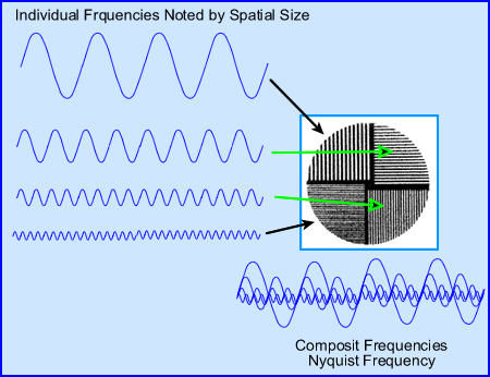
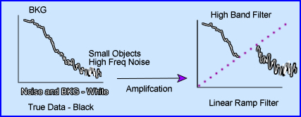
- Furthermore, one must appreciate that the sum (note the above image) of all the frequencies means that there are a lot of different wave patters within NF. In general frequencies can be broken down into
three categories
- Low - background and large objects
- Middle - variation of smaller objects. As the object continue to get smaller the frequency continues to get higher
- High frequencies - small to very small objects plus noise. One cannot differentiate between very small objects and noise because it goes beyond the resolution of the imaging system (FWHM)
- An appropriate sampling for NF is two cycles as noted by the formula below
- The formula identifies the NF to pixel size and the number determines what the actual size the frequency should be in cycles per mm. Let us apply some numbers to see how this works. From our previous work (determining the appropriate pixel size for SPECT) let us revisit the 475 mm FOV
camera
- If we apply the 7.4 mm pixel in the 64 x 64 matrix to the above formula the NF becomes 0.06868 cycles per mm-1
- So what does this mean? This means that in order capture the best spatial frequency the NF must be set at 0.068 cycles/mm-1. To go beyond this point (smaller object) would not improve our resolution
- Note that the pixel value, D, must be twice per cycle it is for that reason that the value is multiplied by 2
- If a 128 matrix is used with a pixel size of 3.7 mm the NF becomes 0.16 cycles/mm-1
- Hence, when you are filtering and reconstructing SPECT data work within its nyquist, but use the whole frequency! And it varies based on magnification and the FOV
- More comments on NF
- Manufacturers define NF in several different ways, two of which are cycles/mm and cycles/pixel
- The above calculations were done in cycles/mm, however, it maybe more appropriate to consider the NF in cycles/pixel
- Why? This is because the maximum NF will always be 0.5 cycles/pixel. The reason for this is that it takes two pixels to capture the entire cycle.
- Therefore, whenever we filter an image in SPECT it is necessary to always capture and work with the entire NF. Failure to not include all of it would result in not capturing all information that is available for processing.
- The images above show the correct NF at 0.5 cycles/pixel, where 2 pixels capture the entire cycle. An example of over sampling is also noted when the NF is set to 1.0 cycles/pixel. What happens if over sampling occurs? (Or try to image higher frequencies) Look below!
A - Shows a set of images taken with different amount of acquired SPECT slices: 16, 32, and 64. Notice the "squares" that can be seen . This Moire type defect is seen more clearly in the background of the transverse slice, but also within the brain phantom. This is known as aliasing. The generation of this artifact is not specifically from over sampling, however, the end result is the same, aliasingB - Shows a set of bars with variation in size. Aliasing, in the center of the image it noted, specifically were the bars just don't line up. This occurred because the NF was set at 1.0 cycles/pixel
Fn Nyquist Frequency D Size of Pixel
- Limited counts in nuclear medicine images always reduces the amplitude of the original image frequency. Collimation, patient to detector distance, type of acquisition orbit, compton scatter, and the reconstruction process all effect image resolution
- The low/high frequencies issues
- The smaller the object
- The fewer the counts the greater the noise and grainy. However, the more the counts the less noise there is. Noise and small objects can become lost in the data which can potential miss disease
- Low end frequency issues might normally be considered background and scatter issues, however, Poisson statistical noise "blurs" or "smooth's" critical data in the low frequency domain, that occurs when reconstruction via backprojection is applied. Also classified in the realm of low frequencies is star defect as discussed in your previous lecture
- The above graph is similar to the previous one, however, there are several differences
- The frequency curves that are displayed include: MTF of the gamma camera (black) with two separately acquired images in red
- From left to right activity on the left contains low frequencies, while that on the right contains high frequencies
- Noise level 1 represents a low count image where noise breaks away midway from the MTF
- Noise 2 represents more counts acquired, when compared to Noise 1. Here the noise level breaks away from the MTF curve further into the higher frequency range
-
One should conclude several points:
- The more counts you acquire the better your resolution via the higher the frequency being image
- Once the red curve breaks from the MTF it is impossible to tell the difference between small objects and noise
- If more counts you acquire the closer the frequency will match the camera's MTF giving you the best possible resolution
- Pre-filtering the raw data
- Many places actually pre-filter the raw rata, which mans that each 2-D image within the 180 or 360 degree rotation is filtered prior to reconstruction. Why?
- The rational for this is simple - If you are dealing with low count images then you're going to have a lot of high frequency noise. By completing a 9-point smooth on each 2-D slice you removing excessive fluctuation in the high frequency range
- Filtering during imaging reconstruction
- When filtering during backprojection and image reconstruction there are several aspects that filters can accomplish
- Removing low frequency (BKG)
- Removing high frequency (noise).
- Low pass filters only allow low to mid frequencies to be processed. This means the exclusion of high frequency data during reconstruction. Example of this might be a Butterworth or Hanning filter
- High pass filters do the opposite. An example of this would include a Ramp filter
- Band pass filter eliminate low and high frequencies and only let mid-range frequencies to be processed
- Restoration filters attempt to restore data and improve the quality of the image. Two examples would include Wiener and Metz
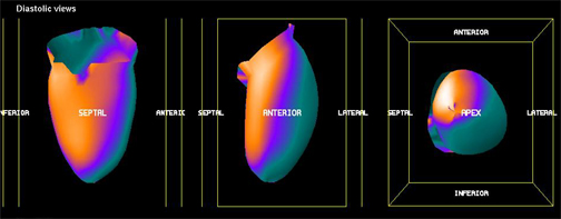
- Partial volume rendering allows the user to create 3-D surface images of an organ that has been acquired through SPECT. Generally, not considered very useful because it does not allow you to look inside the structure. However, analyzing the external anatomy of the brain might lead to finding large "hole" on the brain's exterior surface. This could be due to a lesions or an infarct that affected the brain and included the surface anatomy
- Post-filtering (after reconstruction) is also sometime done, especially if the end results from reconstruction contain a grainy or statistically noisy image. Smoothing the image may be recommended
- Filter the reconstruction with high and low pass filters
- Ramp filter (high pass) - Two issues to consider
- The main role of the linear ramp filter is to amplify the frequency to better resolve the data. However, if the entire frequency was amplified then true counts, bkg, and noise would all be amplified. This would serve no purpose
- Hence, the ramp filter cuts off the low frequency background, which removes unwanted data. This is good! Removing low frequency also removes image blurriness and the star defect
- What remains in are true counts + high frequency noise.
- What do you do with the high frequency noise?
- Adding a low pass filter to the to reconstruction process will can cutoff the noise (Keep this thought in mind)
- Filters and orders
- Some filters allow you to adjust its order. Essentially what that does is change the slope on the filter. In the case above, when you increase the order number on a butterworth filter you increase the negative component of the slope, making it steeper
- This manipulation allows the user to remove or add difference frequencies to the reconstructed image
- Note that an order of 8 increases the amount of lower frequencies, but doesn't accept as many frequencies at the higher end. While decreasing the order number reduces the amount of lower frequencies, but accepts more frequencies
- To accept more lower frequencies and reduce high end creates a more blurry/smooth image. Doing the opposite causes a grainy/noise image
- Yet a second element to all this is considering image contrast. The steeper the slope of the curve the greater the response is to contrast, while a less negative slope has less sensitivity.
- Filters and cut-offs
- Another angle on filters has to do with its cut-off. The examples above show the cut-off frequency set to three different points. Additionally, the MTF response includes the same orders of 2, 4, and 8
- When you set the cut-off that becomes the point at which the reconstructed image no longer accepts the frequency data.
- Note the affects of the different cut-offs above. If you look at 0.4 you can see how it eliminates all the high frequency noise and only a small portion of the patient's data. Of the three cut-offs represented 0.4 would be the most acceptable. Why?
- By adjusting the cut-off we can effective eliminates high frequency noise leaving BKG and true count data. This improving the image quality via the elimination of statistical noise and making the image look more fuzzy/less grainy
- Finally, it is usually recommended that you set the cut-off to 0.5 cycles/pixel. This was mentioned mentioned earlier during the lecture. Why do we want to set the cut-off at 0.5?
- Combining Ramp and Butterworth filters
- The key is to be able to remove as much of the unwanted frequencies as possible. Hence, the application of both low and high filters is required
- The application of Ramp and one of the above low frequency filters is an example of how this process is should work.
- In addition, there are three "globs" of data: BKG, Patient Data, and Noise
- Given the different filters above, which two combinations best removes most of the unwanted data
- Sometimes this application is referred to windowing
- Given the previous image showing four different applications of filters here are two combinations using a low and high band filters. Which of these two combinations is best suited for your filtered reconstructed data?
- Let's spend a little more time discussing other types of filters
- How do restoration filters work?
- The concept is to improve resolution on a low count by restoring counts in an image. Hence, images with low count density may benefit with this type of application
- There are two types that we will discuss: Wiener and Metz
- Application of concept
- Metz filter works similar to ramp in that it amplifies frequencies, but first applies an inverse MTF causing the amplification of low and mid-frequencies instead of the higher frequencies
- The above image shows what happens with the filter that takes the MTF and inverts it. Once this is accomplished the mid and low frequencies are amplified
- Wiener as another type of restoration and it works on a different principle
- It's goal is to filter out noise and it is noise that corrupts the patients counts within the NF
- By applying an SNR concept this filter assumes that signal and noise are linear and its probable distribution can be identified
- Using the statistical concept of "minimum mean-squared error" noise is eliminated from the signal
- Another way to think of this is to assume that the frequency data has multiple convolutions based on the spatial frequencies in an image. THis includes.
- If convoluting noise is identified, then just subtract the deconvolution noise.Or apply a reverse wave/cycle of noise will result in data containing true counts
- Use this hyperlink to find out more about Wiener filters
- Creating a three-dimensional image
- Occasionally someone might want to look at the 3-D surface (surface rendering) of an organ. Examples of this might be the heart or the brain.
- To accomplish this one must a apply a process known as volume rendering
- The most popular type is known as maximum intensity projection (MIP)
- Essentially all transaxial slices are placed on top of each other
- From each row of pixels transferring through all transaxial slices the hottest pixies are identified
- This display shows the LV of the heart which can be manipulation to view any angle with the touch of the mouse. However, it cannot be displayed in this web based program
- Another example of surface rendering shows a brain scan. Ideally this display can be shown as a cine or as a single image where the mouse arrow can be drag to display any angle for the brain
- Most programs allow you to rotate the single picture to any angle the user wishes to look at
- Advantage of this approach is to identify any abnormalities on the surface of the organ
- Disadvantage is simple - you cannot see beyond the surface
- Attenuation correct
- Filters have been designed to take attenuation into account
- The only problem with this approach is that the user can only apply this to areas of the body where the body habitus density remains relatively constant (brain and liver)
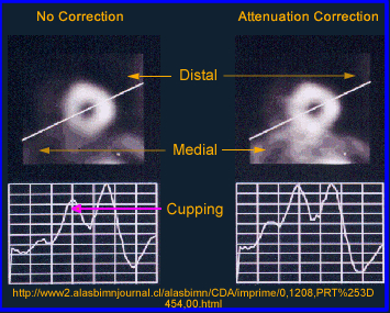
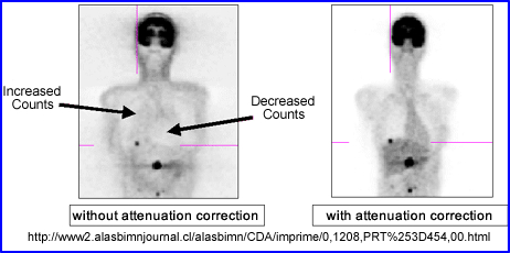
- Why should attenuation be taken into account? Remember the cupping artifact? Graphically the above example shows the affects of cupping in the LV of the myocardium. A profile is drawn through heart and a decreased in counts can be seen in the septal wall. Can you explain this artifact?
- The two types of attenuation filters are used in nuclear medicine: Chang (applied post reconstruction) and Sorenson (applied prior to reconstruction)
- The Chang method starts by drawing an ROI around the widest portion of the transverse slice. Once defined an attenuation value is then given to the data and a correction in counts is applied to the pixels inside the ROI. In theory this increases the counts coming from the center of the image negating the cupping artifac. Remember - the closer to the center of the brain (or any organ) the greater the gamma attenuation and the greater the need for correction
- Water has a µ value of 0.15 cm-1 which is applied to all liver brain and liver attenuation filters
- While attenuation correct filters are sometimes used to improve image quality this process cannot be done if there are different areas of density within the FOV. At this point only a transmission source can be used to compensate for the differences in density within the imaging media. Example of this would include the myocardium ane bone
- Transmission imaging can be accomplished with the use of a line source and a fan beam collimator or with an x-ray tube (CT)
Return to the beginning of the document
Return to the Table Of Contents - How do restoration filters work?
|
 |
|---|
Chapter 10, The Essential Physics of Medical Imaging,Bushberg Radiation Detection and Measurement, Knoll, 2nd ed. http://engineering.dartmouth.edu/courses/engs167/11%20Image%20Analysis.pdf