For most of you this is a review (CLRS 322) and my intent is not to overwhelm you in this ares since it has already been covered. So if the material below looks familiar it is. So go over this material, it's a good refresher in an area in nuclear medicine that really isn't that easy to understand. Keep in mind the following points:

• How SPECT imaging applies filtered reconstruction. It's the same application in PET.
• While SPECT tends to use Filtered Backprojection (FBP) for reconstruction. PET applies Iterative Reconstruction (IR).
• The question is why IR over FBP? First look at a PET phantom and notices the amount of arrays emanating from it when FBP is used. In the same link you can see that those lines are lost when IR is applied.
• PET tends to image a lot of "hot spots," caused the streaking artifacts (LORs). Are these streaks low or high frequencies?
• For this reason IR is the preferred method for image reconstruction.
• When you apply reconstruction filter or filters your goals are: remove background and eliminate the noise (as much as possible) thus improving image contrast.

1. Frequencies
1. Ideally a filter's role is to enhances image quality, without significantly altering the raw components of the input data
1. Incorrect filtering, over/udder process the reconstruction data effecting image quality by: reducing resolution or contrast, increase noise (high frequency), increase background counts (low frequency), and can blur or over sharpen detailed information. The image may become either too grainy or too blurry
2. Goal - Enhance the true counts and remove the undesirables: background and noise
3. You may recall that SPECT images generally have fewer less counts, however in PET, there is a more "count rich" acquisition that applies a 128 matrix is used. When acquiring a SPECT which matrix is the most common?
2. In PET, image filtering requires the conversion of spatial to the frequency domain.
   1. Consider the acquisition of PET data as a form of digital sampling. You are collecting only a sample of data as the image is acquired around the patient
   2. For the camera to resolve the incoming data many factors must be considered: sinograms, TOF, scatter/random, attenuation, attenuation correction, and count density per voxel
   3. That said, our focus should be on how the computer converts the spatial domain (counts) to the frequency domain. This is done with the use of Fourier Transform method (if you want to review additional material, which was covered in CLRS 322 click the link)

       

   
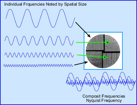
   4. Let us take a look at the what happens when spatial is converted to frequency In general, frequencies can be broken down into different categories. Let us consider
      1. Low - background and large objects
      2. Middle - variation of smaller objects. As the object continue to get smaller the frequency continues to get faster and shorter
      3. High frequencies - small to very small objects plus noise. One cannot differentiate between smallest objects and noise because it goes beyond the resolution of the imaging system (FWHM)
   5. When we talk about frequencies one must also consider the Nyquist Frequency (NF)

   Fn	Nyquist Frequency
   D	Size of Pixel

   6. The formula associates the NF to pixel size determines the actual size the frequency in cycles per mm. Let us apply some numbers to see how this works.
      1. If we have a 7.4 mm pixel in the 64 x 64 matrix and apply it to the above NF formula then this value is 0.06868 cycles per mm^-1
      2. So what does this mean? This means that in order capture the best spatial frequency the NF must be set at 0.0687 cycles/mm^-1. To go beyond this point or an attempt to find smaller objects would not improve our resolution
      3. If a 128 matrix is used with a pixel size becomes 3.7 mm then the NF becomes 0.135 cycles/mm^-1
      4. The result of a 128 matrix means more cycles per mm, better resolution
      5. Hence, when you reconstructing an image and applying filters with SPECT or PET data must be within its Nyquist and the user should apply the entire frequency!
   7. More comments on NF
      1. Manufacturers define NF in several different ways, two examples are cycles/mm and cycles/pixel
      2. The above calculations were done in cycles/mm, however, it maybe more appropriate to consider the NF in cycles/pixel
      3. Why? Because the maximum NF should always be 0.5 cycles/pixel. The reason for this is that it takes two pixels to capture the entire cycle.
      

   8. Therefore, whenever we filter an image in SPECT or PET it is necessary to always capture and work with the entire NF. Failure to not include all of it would result in not capturing all the data that is available for processing
      1. The images above show the correct NF at 0.5 cycles/pixel, where 2 pixels capture the entire cycle. An example of over sampling is also noted when the NF is set to 1.0 cycles/pixel. What happens if over sampling occurs? (Or try to image higher frequencies) Look below!
      2. Any time you go beyond 0.5 cycles/pixel aliasing occurs
      
      
      A - Shows a set of images taken with different amount of acquired PET slices: 16, 32, and 64. Notice the "squares" that can be seen . This Moire type defect is seen more clearly in the background of the transverse slice, but also within the brain phantom, i.e. aliasing.

      B - Shows a set of bars with variation in size. Aliasing, in the center of the image as noted, specifically were the bars just don't line up. This occurred because the NF was set at 1.0 cycles/pixel

2. What's in the frequency?

1. Limited counts in nuclear medicine images always reduces the amplitude of the original image frequency. Collimation, patient to detector distance, type of acquisition orbit, Compton scatter, and the reconstruction process all effect image resolution
2. The low/high frequencies issues
   1. Smaller objects can be captured, however, as an object continues to get smaller it will eventually blends in with noise
   2. The fewer the counts the greater the noise and more grainy an image will be
   3. Low end frequency issues might normally be considered, background and scatter, however, Poisson statistics "blurs" or "smooths" critical data in the low frequency domain, this occurs when reconstruction via Backprojection is applied. Also classified in the realm of low frequencies is the star defect



3. The above graph is similar to the previous one, however, there are several differences
   1. The frequency curves that are displayed include: MTF of the gamma camera (black) with two separately acquired images in red
   2. From left to right activity on the left contains low frequencies, while that on the right contains high frequencies
   3. Noise level 1 represents a lower count image where noise breaks away midway from the MTF
   4. Noise 2 represents more counts acquired, when compared to Noise 1. Here the noise level breaks away from the MTF curve further into the higher frequency range
   5. One should conclude several points:
      1. The more counts you acquire the better your resolution via the the ability to see higher frequencies (smaller objects)
      2. Once the red curve breaks away from the MTF it is impossible to tell the difference between small objects and noise
      3. If more counts are acquired you can push the red-line further down the MTF, improving resolution
3. Filters Application
1. Pre-filter the raw data
   1. Many places actually pre-filter the raw data, which means that each 2-D image within the 180 or 360 degree rotation is filtered prior to reconstruction. Why?

   

   2. The rational for this is simple - If you are dealing with low count images then you're going to have a lot of high frequency noise. By completing a 9-point smooth on each 2-D image you removing excessive fluctuation in the high frequency range
2. Filtering during imaging reconstruction
1. When filtering during Backprojection and image reconstruction two points can work towards image quality
   1. Removing low frequency (BKG)
   2. Removing high frequency (noise).
2. Low pass filters only allow the passing of low to mid frequencies, whereas, high frequency data is removed. Examples of these types of reconstruction filters would include Butterworth or Hanning filter
3. High pass filters do the opposite. An example of this would be a Ramp filter
4. Band pass filter eliminate low and high frequencies and only allow mid-range frequencies to be processed
5. Restoration filters attempt to restore data and improve the quality of the image. Two examples would include Wiener and Metz
6. Partial volume rendering reconstruction filters allows the user to create 3-D surface images of an organ. However, it generates the edge of the object where the activity starts to build up. on the down slide you cannot look beyond the surface. Analyzing the external anatomy of the brain might lead to finding large "hole" on the brain's exterior surface
7. Post-filtering (after reconstruction) is also sometime done, especially if the end results from reconstruction contain a grainy or statistically noisy image.
3. Filter the reconstruction with high and low pass filters
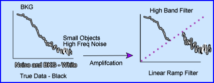
1. Ramp filter (high pass) - Two issues to consider



1. The main role of the linear ramp filter is to amplify the frequency to better resolve the data. However, if the entire frequency was amplified then true counts, bkg, and noise would all be amplified. This would serve no purpose
2. Hence, the ramp filter cuts off the low frequency background, which removes unwanted data. This is good! Removing low frequency also removes image blurriness and the star defect
3. What remains in are true counts + high frequency noise.
4. So what do you do with the high frequency noise?
5. Adding a low pass filter to the to reconstruction process will cutoff the noise (Keep this thought in mind)
2. Filters and orders

1. Some filters allow you to adjust its order. Essentially what that does is change the slope on the filter. In the case above, when you increase the order number on a Butterworth filter you increase the negative component of the slope, making it steeper
2. This manipulation allows the user to remove or add difference frequencies to the reconstructed image
3. Note that an order of 8 increases the amount of lower frequencies, but doesn't accept as many frequencies at the higher end. While decreasing the order number reduces the amount of lower frequencies, but bring in more high frequencies
4. To accept more lower frequencies and reduce high creates a more blurry/smooth image. Doing the opposite causes a grainy/noise image
5. Another element to Butterworth is the manipulation of image contrast. The steeper the slope of the curve the greater the response is to contrast, while a less negative slope has less sensitivity you are to image contrast
3. Filters and cut-offs

1. Another angle on filters has to do with its cut-off. The examples above show the cut-off frequency set to three different points. These MTF curves includes the same orders of 2, 4, and 8
2. Setting the cut-off means that anything beyond is rejected
3. Note the affects of the different cut-offs above. With a cutoff of 0.4 and an order of 6 or 8 means that you will eliminate all data past its point. Of the three cut-offs represented 0.4 would be the most acceptable. Why?
4. By adjusting the cut-off we can effective eliminates high frequency noise leaving BKG and true count data. This improving the image quality via the elimination of statistical noise and making the image look more fuzzy/less grainy
5. Finally, it is usually recommended that you set the cut-off to 0.5 cycles/pixel.
4. Combining Ramp and Butterworth filters
1. The key is to be able to remove as much of the unwanted frequencies as possible. Hence, the application of both low and high filters is required



2. The application of Ramp and one of the above low frequency filters is an example of how this process should work
3. In addition, there are three "globs" of data: BKG, Patient Data, and Noise
4. Given the different filters above, which two combinations best removes most of the unwanted data and saves most of the true data?
5. When low and high frequency filters are used together this is referred to as windowing
6. Given the previous image showing four different applications of filters here are two combinations using a low and high band filters. Which of these two combinations is best suited for your filtered reconstructed data?
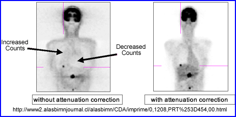
5. Attenuation correction
   1. Filters have been designed to take attenuation into account
   2. The only problem with this approach is that the user can only apply this to areas of the body where the body habitus density remains relatively constant (brain and liver)
   
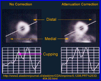
   3. Why should attenuation be taken into account? Remember the cupping artifact? Graphically the above example shows the affects of cupping in the LV of the myocardium. A profile is drawn through heart where decreased counts can be seen in the septal wall. Can you explain this artifact?
   4. The two types of attenuation filters used in nuclear medicine: Chang (applied post reconstruction) and Sorenson (applied prior to reconstruction)
   5. The Chang method starts by drawing an ROI around the widest portion of the transverse slice. Once the attenuation value is in place then given the filter can correct the for the lost counts with the ROI. In theory this increases counts coming from the center of the image negating the cupping artifact. Remember - the closer to the center of the brain (or any organ) the greater the gamma attenuation and the greater the need for correction
   
   6. While attenuation correct filters are sometimes used to improve image quality this process cannot be done if there are different areas of density within the FOV. At this point only a transmission source can be used to compensate for the differences in density within the imaging media. Example of this would include the myocardium and bone
   7. Transmission imaging can be accomplished with the use of a line source and a fan beam collimator or with an x-ray tube (CT), but in today's technology one almost always uses CT

---

Iterative Reconstruction

1. Iterative methods (IR) - Is an alternative process to FBP reconstruction that continues to gain popularity in Nuclear Medicine. The area where IR is currently be utilized the most is in PET, however, its application can be seen in general nuclear medicine as well
2. This reconstruction method employees the following:
1. Attenuation correction map can be employed in the IR process
2. Estimation of radiopharmaceutical distribution occurs
3. Uniform distribution of activity may be applied or
4. Backprojection measurements from an applied matrix can be utilized
5. Employs imaging physics
3. When compared with FBP, IR improved distribution of data, hence quantitative analysis becomes a reality with PET
1. IR does not apply the sum of the arrays, therefore there is is NO star defect
2. Based on all the points made above quantification of data, such as SUVs, can be conducted
4. Iterative methods requires intensive computer processing that is available with current CPU technology. Years ago iterative reconstruction was not practical because CPU processors were too slow
5. The following example is a "simple explanation" of the Iterative reconstruction process. Note that the diagram is numbered to match the explanation below

1. Data is acquired in a set of 2D sinograms 360 degrees around the patient
2. Prior to IR the original matrix maybe filtered (smoothed) to reduces statistical noise
3. (1) The Initial Guess comes from
   1. The expected biodistribution of the radio-tracer
   2. This may be obtained from one of several methods: (a) assume a uniform distribution of activity or (2) apply data from all the 2D Backprojection images
4. (2) A forward projection step then generates an Estimated 3D Matrix which is influenced by the patient's attenuation map and extra data usually specific to imaging physics
5. (3) Then all 2D Estimated Projections (or sinograms) are compared to the 2D Measured Projections (sinograms) where variation are identified
6. (4) This generates a 3D Error Matrix which then updates step 2 (estimated 3D matrix)
7. (2) Estimated 3D Matrix is modified creating a new Estimated 3D Matrix
8. The cycle then starts over again hence the term iterative
9. The user defines the amount of iterations necessary to complete image reconstruction
10. Each iteration brings a "truer" count to each voxel
11. In the end, the estimated 3D matrix should closely match the "true count" distribution in the 3D structure
6. Types of Iterative algorithm
   1. Expectation Maximization (EM) is the overall terminology used for define IR programs
      1. This example is the initial one explained in today's lecture
      2. Forward projection step is the expected operation and the comparison step is the maximization operation
      3. Then the Backprojection step creates the error matrix and this updates the estimated 3D matrix
   2. Maximum-Likelihood (MLEM) - move involved
      1. This algorithm compares the the estimated to measured activity
      2. The process maximizes the statistical quantity, referred to as likelihood, between the estimated and the expected
      3. The closer the value is to 1 the better its representation of true counts
      4. End results - to generate the greatest probability of measured activity that truly represents the actual counts
      5. Evaluates and processes ALL projections in each iteration
      6. It may take between 50 to 100 iterations to complete the reconstruction process (this is very time consuming)
   3. Ordered-Subset (OSEM)
      1. To reduce the processing time the projections are broken down into subsets and then processed at that sub level
      2. As an example if 128 projections are acquired they might be broken down into 8 subsets where each subset containing 16 projection
      3. Each estimated subset is then compared to its measured (acquired) counterpart (subset) which then updates it to a new estimated subset
      4. Each subset goes through multiple iterations
      5. In this example, 8 subsets are handled individually, compared and updated, which when, combination represent the new estimated 3D matrix
      6. Usually no more than 10 iterations with each subset
   4. A problem with noise
      1. For each iteration noise is generated. This is referred to as "noise breakup phenomenon"
      2. Hence, there is a compromise between an image that shows the best detail and has the least amount of noise
      3. If the iterative process continued excessively, then too much noise would be noted in the image
      4. Post-filtering with a smoothing filter may be considered to suppress the noise created in the IR process
7. What needs to be appreciated is that each iteration gets you closer estimate to the true count distribution in the 3D matrix. On the negative side the more iterations generate more noise.



8. Several improvements occur with the iterative process: loss of the star defect, improved resolution, and better image contrast

9. The above example shows how increasing the amount of iterations improves image quality by better estimating the true count distribution in the SPECT procedure. When do you think the iterations should be stopped? 15?

Return to the beginning of the document
Return to the Table Of Contents

2/23

Chapter 10, The Essential Physics of Medical Imaging,Bushberg Radiation Detection and Measurement, Knoll, 2nd ed. http://engineering.dartmouth.edu/courses/engs167/11%20Image%20Analysis.pdf