Example 4: Estimating Intersection Points and Shading Regions for Inequalities

Objectives: To graphically estimate the intersection point of two curves, and to shade solutions regions for inequalities

Example 4A: Using DPGraph, graphically estimate the points of intersection of the curves ln(x) and cos(x).

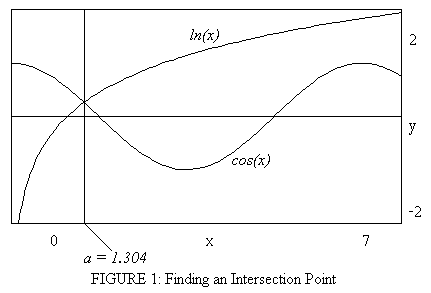
Click here to download the .dpg file. The range for x, namely, from 0 to 7 is chosen to show that ln(x) clears the maximum of cosine after the first intersection point. Hence there can be only one intersection point between the two curves. This is illustrated in Figure 1 below:

In the last line of the .dpg file, notice the equation x = a. This plots a vertical line through the plot at the value specified in the file for the value a. Using the scrollbar, change the value of a, thus moving the vertical line until it passes through the intersection point. The value of a at this point is given at the bottom of the DPGraph screen and noted in Figure 1. Based on this estimate, we may conclude that the equality ln(1.304) = cos (1.304) holds approximately (to two decimal places according to the calculator with cosine computed in radian mode).

Example 4B: Graph the domain of the function

z = f(x,y) = ln(4(x^2 + y^2) - 2(x + y) - x^4 - y^4)).

Since the function ln(..) is defined only when inside the parentheses is positive, we need to graph the following main inequality:

4(x^2 + y^2) - 2(x + y) - x^4 - y^4 > 0

This is easily done with the DPGraph. Click here for the .dpg file, which produces the following graph:

In the last line of the .dpg file, note the inequality z < 0 that is separated by "&" from the main inequality. This z inequality is responsible for the "shading" while the boundary of the shaded region is determined by the main inequality. All the white areas, including the circular hole, represent regions where the main inequality does not hold.