DPGraph
![]()
DPGraph (Dynamic Photorealistic Graphing) has many easy to use features which I won't go through here (but check the Notes below). The features I would like to emphasize and discuss here are the following:
The scrollbar and its usefulness in studying stability and bifurcations in one-parameter families of maps;
Creating bifurcation diagrams easily using the implicit graphing capabilities of DPGraph.
As this is not meant to be a tutorial, I will skip the operational details of the software for now.
The scrollbar and one-parameter families of maps.
Basically, the scrollbar is a tool with which a parameter in a given function, or equation, can be changed while you are looking at the also changing graph of that equation. You will see how the graph changes as you change the parameter; the faster your machine, the smoother the changes. So suppose you are studying, or teaching about, a one-parameter family of maps of the real line. You enter the map's formula just as it is, with the parameter called "a", and manipulate the formula using the scrollbar. Take the familiar logistic map, for instance. Enter its equation in the "graph3d" command as:
y = ax(1-x)
If you'd like to see the coordinate axes and the identity line, you can add them in as follows:
y = ax(1-x), y = x, y = 0, x = 0
Now "execute" to see a graph pop out, like the one below:
Here the parameter value is set at a = 3.5. The vertical line through the nonzero fixed point shows how to use the scrollbar to estimate things like fixed points, critical points, etc. Add
x = b
to the above list of equations, where b is a second DPGraph parameter. Use the scrollbar to change b, thus moving the vertical estimator line until it is visually best aligned with the fixed point. Read the value of b at the bottom of DPGraph screen and you'll have a good first estimate of the location of the fixed point! You may get rid of the estimator line once you finish estimating the fixed point, and if greater precision of the estimate is desired, the DPGraph estimate provides a splendid first "guess" in a Newton method like algorithm.
Now change a and see the logisitc map modified accordingly, right in front of you on the screen. The graph below shows some snapshots of this process corresponding to integer values of a from 1 (lowest curve) to 5 (tallest):
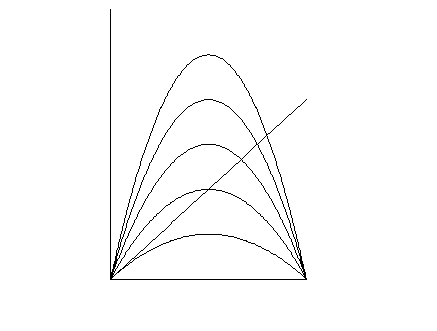
It is important to realize that this modification of the graph takes place dynamically while moving a Windows bar (see Note 2 below). To get the above graph, once you identify the a values of interest, just add all the corresponding equations (instead of the original one with the a) to the above list and DPGraph will plot all of them simultaneously in the same coordinate system. You may also annotate and print them by copying the graph to the clipboard and then pasting it into an application such as the MS Paint or similar.
Next, suppose that you want to find the period-2 points. If you add to the above list of equations, the following
y = a(ax(1-x))(1-ax(1-x))
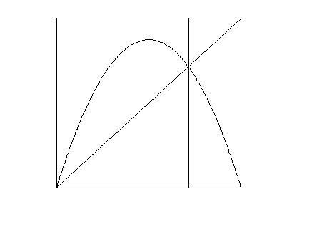
which is just the logistic map f(x) composed with itself once, then you'll see the graphs of the logistic and its iterate f(f(x)) together, as in the following diagram:
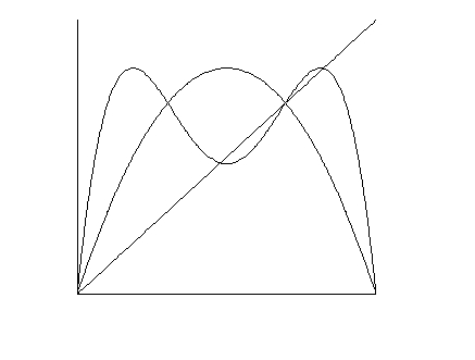
From the above diagram (where a = 3.3) you can estimate the location of period-2 points, namely the intersection points of f(f(x)) with the identity line, the same way the fixed point was estimated using a moving estimator line (here they are 0.48 and 0.82, approximately). Also, by changing the logistic parameter a, you can see the "birth" of 2-cycles and the changing stability characteristics of the nonzero fixed point. The latter is reflected, as some may know (or see Note 3 below), in the way the graph of f(f(x)) crosses the identity line at the fixed point. Here we see that the fixed point at a = 3.3 is in fact unstable since f(f(x)) lies below y = x on the left and above it on the right. Of course, to the extent that it is reliably possible, you may also tell about the stability by visually checking the slope of the curve through its intersection points with the identity line (DPGraph keeps the same scale on both coordinate axes in the full screen mode). For example, looking at the slope of f(f(x)) which seems to have a magnitude of less than unit through the period-2 points in the last graph above, we may conclude that the 2-cycle is attracting. See Note 2 below for a movie showing the birth of the 2-cycle dynamically!
Clearly, any function f may be graphed, together with one or two iterates (perhaps to see about 2- and 3-cycles). The scrollbar can be used to study one-parameter family of maps as outlined above.
Creating bifurcation diagrams (the one-parameter case).
The preceding discussion shows us where (locations where some iterate of f(x) intersects y = x) and how (tangent, period-doubling or other) bifurcations occur as we change the value of the parameter a with the scrollbar. Using the implicit graphing feature of DPGraph, we can do more.
As a rule, DPGraph 2000 implicitly graphs equations, with functions as particular cases. Bifurcation curves are solutions of equations, so they can be easily graphed also. For example, if we define
F(x,a) = ax(1-x)
then the solution of the equation
F(x,a) = x
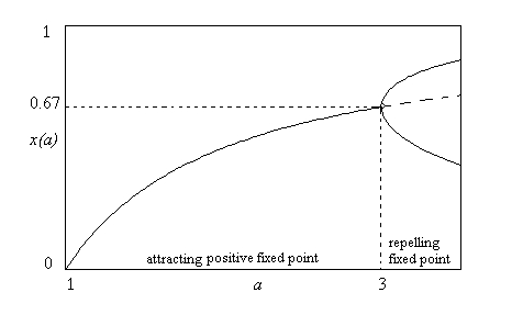
which can be expressed as x = x(a), gives the locus of the fixed points of the one-parameter family as a function of the parameter a. Although we may not be able to determine the bifurcation curve x(a) analytically in all cases, it is a simple matter to graph it, and then analyze the graph. A similar comment applies to the iterates of maps. For instance, the solution x(a) of the equation
f(f(x)) = a(ax(1-x))(1-ax(1-x)) = x
shows the period-doubling bifurcation of a 2-cycle, as in the diagram below:
In the above figure, the a values are plotted on horizontal axis and the x values are on the vertical axis. Since DPGraph uses the letters x and y for the horizontal and the vertical axes, respectively, we need to switch a in the above equation to x, and x to y; i.e., we need to enter the following equation in the "graph3d" command:
x(xy(1-y))(1-xy(1-y)) = y
and it is the graph of this equation that is actually shown in the bifurcation diagram above (the annotations, labelings and dash/dotting were done in MS Paint). Similarly, the solution (according to the above procedure) of
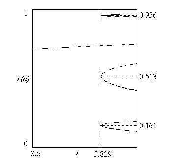
f(f(f(x))) = aa(ax(1-x))(1-ax(1-x))(1-a(ax(1-x))(1-ax(1-x))) = x
shown below illustrates the tangent bifurcation of both the attracting and repelling 3-cycles:
Two-parameter bifurcation sets and surfaces.
Things get more complicated when two parameters are involved. Bifurcation curves turn into surfaces, and bifurcation points into sets or curves. As a sampler, we study the "canonical" example of cusp bifucation (also known as the "elementary cusp catastrophe"). For one-dimensional maps, this involves a third dergree polynomial map with two parameters, say, a and b, such as
f(x) = f(x;a,b) = x^3 + ax + b = 0,
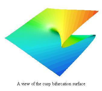
where the term ax subsumes a "-x" term taken to the left side from right. The above equation defines a surface implicitly in the three dimensional space, which may be plotted with the DPGraph as follows:
z^3 + xz + y = 0,
where we plot the a parameter on the x-axis, the b parameter on the y-axis, and the fixed point locus x is represented as the z variable. The surface is plotted below:
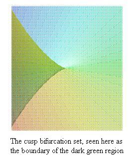
When we view this surface from the top (equivalently, project the surface onto the xy- or ab-plane) and increase graph transparency in DPGraph's edit menu to see through the surface, we get the following diagram:
which explains the name "cusp" rather clearly. As is obvious from the surface, the blue regions lie lower than the red regions.
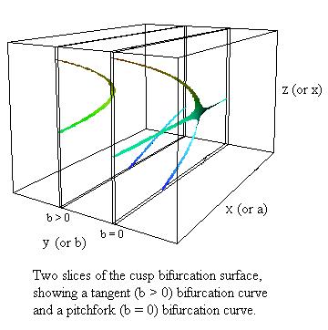
When b is fixed, we get a one-parameter cubic equation, which depending on the values of the remaining parameter a, displays either tangent bifurcations or, exceptionally when b = 0, a "pitchfork" bifurcation. The corresponding bifurcation curves are easily visualized as the cross sections, or "slices" of the bifurcation surface. Such slices are obtained in DPGraph using the scrollbar; the following diagram shows two such slices:
Three parameter bifurcation sets and hypersurfaces.
Because of the scrollbar and animation features of DPGraph, we may dynamically sketch level surfaces of the hypersurface that represents a 3-parameter family of one-dimensional maps. For example, consider the canonical 3-parameter bifurcation equation
f(x) = f(x;a,b,c) = x^5 + ax^3 + bx + c = 0
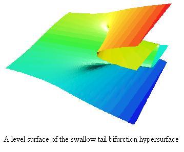
called the "swallow tail" bifurcation hypersurface, or more commonly, the swallow tail "catastrophe". To graph a level surface of this hypersurface in DPGraph, we plot:
z^5 + x(z^3) + dz + y = 0
where the DPGraph parameter "d" takes the place of the 4-th variable and is used to define a particular level surface. Naturally, here x represents a, y is c and z is x; the following graph shows the level surface corresponding to a given value of d:
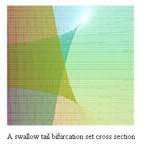
To gain a more comprehensive understanding of the swallow tail hypersurface, we may switch roles and use, e.g., x for b and d for a, and so on. We may also project this level surface onto the xy- or here, the ac-plane, as in the case of cusp bifurcation to get:
In this diagram, we see a double-cusped, swallow tail configuration. It is possible to animate the preceding level surface, or its analogs, to see the 4 dimensional hypersurface as a 3 dimensional movie of its level surfaces; see the following notes.
NOTES.
DPGraph is an inexpensive, reliable and easy to use software created by David Parker. It is very fast and takes up little space on your hard-drive. As I mentioned earlier, DPGraph does many things that I haven't talked much about here. In fact, its strong point is 3D implicit surface graphing with attractive photorealistic rendering, a small glimpse of which is seen in the surface graphs above. The ease of use, quality of graphs and availibility of free updates are exceptional for such an inexpensive software. Many useful examples and interesting graphs are found on the internet homepage of the software and in the various links that are listed there. To examine some of these examples or links, and to acquire a copy of DPGraph, click here and follow the easy instructions to download and install the software.
If a copy of DPGraph is installed on your machine, then you can run interactive sessions in which you can change the parameter value a as discussed above or see a movie about the birth of a 2-cycle and do much the same things with any mapping, not just the logistic. This could also be a good tutorial session if you are new to DPGraph, in which case, I recommend saving the .dpg files on your hard drive for later use and/or modification (that way, it is not necessary to remember all the commands required to generate 2D graphs formatted as above). Here are three logistic files, and a swallow tail movie for starters:
Graphical Analysis Click the link to get the graphs of the logistic map and its first two iterates; using the scrollbar to change the parameter value a, you will see how first a 2-cycle (by period-doubling) and then a 3-cycle (by tangency) is born, and at which parameter values.
Bifurcation Curves Click the link to get the graph of the bifurcation curves for both 2 and 3-cycles; by modifying the equations, bifurcation curves for other mappings can easily be obtained.
A Cycle is Born Click the link to see a movie on how a fixed point spawns two period-2 points as the value of a increases (see the "Help" files of DPGraph for aid in constructing similar movies for other maps or periods).
Swallow Tail Hypersurface Click the link to see a movie where level surface cross sections move up and down to reveal the hypersurface in space-time! For more on how to graph surfaces, animated or not, you may visit any of the links on DPGraph's home page mentioned above.
For more details on how f(f(x)) is used to determine the stability of fixed points, or other questions, click here to send me an email.
(Last update by H. Sedaghat: May, 2001)